相机模型和非线性优化
一、图像去畸变
现实生活中的图像总存在畸变。原则上来说,针孔透视相机应该将三维世界中的直线投影成直线,但是当我们使用广角和鱼眼镜头时,由于畸变的原因,直线在图像里看起来是扭曲的。本次作业,你将尝试如何对一张图像去畸变,得到畸变前的图像。
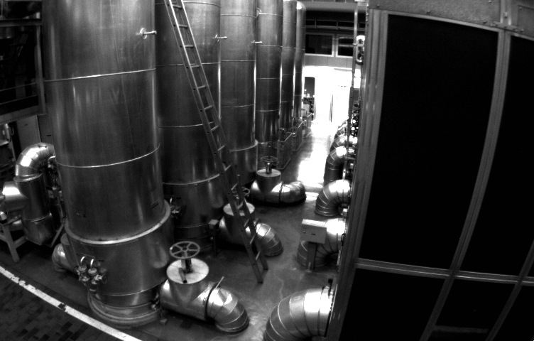
图1. 畸变图片
图 1 是本次习题的测试图像(code/test.png),来自 EuRoC 数据集 [1]。可以明显看到实际的柱子、箱子的直线边缘在图像中被扭曲成了曲线。这就是由相机畸变造成的。根据我们在课上的介绍,畸变前后的 坐标变换为:
\(\left\{\begin{matrix} x_{distorted} = x(1 + k_1r^2 + k_2r^4)+ 2p_1xy + p_2(r^2 + 2x^2) \\ y_{distorted} = y(1 + k_1r^2 + k_2r^4)+ p_1(r^2 + 2y^2)+ 2p_2xy \end{matrix}\right.\)
其中 x,y 为去畸变后的坐标,\(x_{distorted}\),\(y_{distroted}\) 为去畸变前的坐标。现给定参数:
\(k_1 = −0.28340811, k_2 = 0.07395907, p_1 = 0.00019359, p_2 = 1.76187114e−05.\)
以及相机内参
\(f_x = 458.654,f_y = 457.296,c_x = 367.215, c_y = 248.375\)
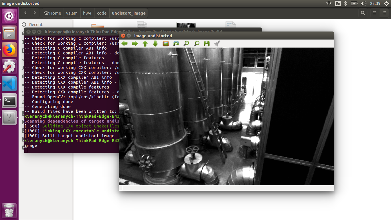
请根据 undistort_image.cpp 文件中内容,完成对该图像的去畸变操作。 注:本题不要使用 OpenCV 自带的去畸变函数,你需要自己理解去畸变的过程。
CODE:
// TODO 按照公式,计算点(u,v)对应到畸变图像中的坐标(u_distorted, v_distorted) (~6 lines)
// start your code here
double x, y, r2, r4, x_distorted, y_distorted;
x = (u - cx)/fx;
y = (v - cy)/fy;

r2 = x*x + y*y,
r4 = r2*r2;

x_distorted = x*(1 + k1*r2 + k2*r4) + 2*p1*x*y + p2*(r2 + 2*x*x);
y_distorted = y*(1 + k1*r2 + k2*r4) + p1*(r2 + 2*y*y) + 2*p2*x*y;

u_distorted = fx*x_distorted + cx;
v_distorted = fy*y_distorted + cy;
// end your code here
二、双目视差的使用
双目相机的一大好处是可以通过左右目的视差来恢复深度。课程中我们介绍了由视差计算深度的过程。 本题,你需要根据视差计算深度,进而生成点云数据。本题的数据来自 Kitti 数据集 [2]。
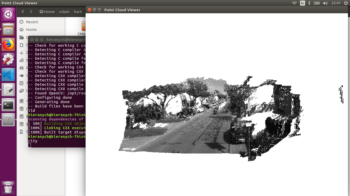
Kitti 中的相机部分使用了一个双目模型。双目采集到左图和右图,然后我们可以通过左右视图恢复出 深度。经典双目恢复深度的算法有 BM(Block Matching), SGBM(Semi-Global Block Matching)[3, 4] 等, 但本题不探讨立体视觉内容(那是一个大问题)。我们假设双目计算的视差已经给定,请你根据双目模型, 画出图像对应的点云,并显示到 Pangolin 中。
本题给定的左右图见 code/left.png 和 code/right.png,视差图亦给定,见 code/right.png。双目的参 数如下:
\(f_x = 718.856, f_y = 718.856, c_x = 607.1928, c_y = 185.2157.\)
且双目左右间距(即基线)为:
\(d = 0.573 m\)
请根据以上参数,计算相机数据对应的点云,并显示到 Pangolin 中。程序请参考 code/disparity.cpp 文件
// start your code here (~6 lines)
// 根据双目模型计算 point 的位置
uchar disp= disparity.at<uchar>(v, u);
point[2] = (fx*d)/disp;
point[1] = point[2]*(v - cy)/fy;
point[0] = point[2]*(u - cx)/fx;

pointcloud.push_back(point);
// end your code here
三、矩阵运算微分
在优化中经常会遇到矩阵微分的问题。例如,当自变量为向量 x,求标量函数 u(x) 对 x 的导数时,即为矩阵微分。通常线性代数教材不会深入探讨此事,这往往是矩阵论的内容。我在 ppt/目录下为你准备了 一份清华研究生课的矩阵论课件(仅矩阵微分部分)。阅读此 ppt,回答下列问题:
设变量为 \(x∈R^N\),那么:
1.矩阵 \(A∈R^{N\times N}\),那么 \(\frac{d(Ax)}{dx}\) 是什么?
由题,可设
\(A=\begin{bmatrix} a_{11} & a_{12} & \cdots & a_{1n}\\ a_{21} & a_{22} & \cdots & a_{2n}\\ \vdots & \vdots & \ddots & \vdots\\ a_{n1} & a_{n2} & ... & a_{nn} \end{bmatrix}\) , \(x = \begin{bmatrix} x_{1}\\ x_{2}\\ \vdots\\ x_n \end{bmatrix}\),
则
\(Y = Ax = \begin{bmatrix} a_{11}x_1 + a_{12}x_2+\cdots + a_{1n}x_n \\ a_{21}x_1 + a_{22}x_2+\cdots + a_{2n}x_n\\ \vdots\\ a_{n1}x_1 + a_{n2}x_2+\cdots + a_{nn}x_n \end{bmatrix}\) ,
\(\frac{d(Ax)}{dx} =\frac{d(Y)}{dx} = \begin{bmatrix} \frac{\partial y_1}{\partial x_1}& \frac{\partial y_2}{\partial x_1} & \cdots & \frac{\partial y_n}{\partial x_1}\\ \frac{\partial y_1}{\partial x_2}& \frac{\partial y_2}{\partial x_2} & \cdots & \frac{\partial y_n}{\partial x_2} \\ \vdots & \vdots & \ddots & \vdots\\ \frac{\partial y_1}{\partial x_n}& \frac{\partial y_2}{\partial x_n} & \cdots & \frac{\partial y_n}{\partial x_n} \end{bmatrix} = \begin{bmatrix} a_{11} & a_{21} & \cdots & a_{n1}\\ a_{12} & a_{22} & \cdots & a_{n2}\\ \vdots & \vdots & \ddots & \vdots\\ a_{1n} & a_{2n} & ... & a_{nn} \end{bmatrix} = A^T\)
2.矩阵 \(A∈R^{N\times N}\),那么 \(\frac{d(x^TAx)}{dx}\) 是什么?
由题可设
\(Y = x^T\begin{bmatrix} a_{11}x_1 + a_{12}x_2+\cdots + a_{1n}x_n \\ a_{21}x_1 + a_{22}x_2+\cdots + a_{2n}x_n\\ \vdots\\ a_{n1}x_1 + a_{n2}x_2+\cdots + a_{nn}x_n \end{bmatrix} \\ = x_1(a_{11}x_1 + a_{12}x_2+\cdots + a_{1n}x_n) + x_2(a_{21}x_1 + a_{22}x_2+\cdots + a_{2n}x_n) \\ = + \cdots + x_n( a_{n1}x_1 + a_{n2}x_2+\cdots + a_{nn}x_n) \\ = \sum_{i=1}^n\sum_{j=1}^n x_i(a_{ij}x_j)\)
则,
\(\frac{d(x^TAx)}{dx} = \begin{bmatrix} \frac{\partial z}{\partial x_1} & \frac{\partial z}{\partial x_2} & \cdots & \frac{\partial z}{\partial x_n} \end{bmatrix}^T\)
其中 \(\frac{\partial z}{\partial x_k} = \sum_{i=1}^n a_{ik}x_i + \sum_{j=1}^na_{kj}x_j\),
所以 \(\frac{d(x^TAx)}{dx} = A^Tx\)
3.证明: \(x^TAx = tr(Axx^T)\).
证明:
\(x^TAx = \sum_{i=1}^n\sum_{j=1}^n x_i(a_{ij}x_j)\)
\(Axx^T = \begin{bmatrix} a_{11}x_1 + a_{12}x_2+\cdots + a_{1n}x_n \\ a_{21}x_1 + a_{22}x_2+\cdots + a_{2n}x_n\\ \vdots\\ a_{n1}x_1 + a_{n2}x_2+\cdots + a_{nn}x_n \end{bmatrix}x^T \\ =\begin{bmatrix} x_1\sum_{i=1}^{n}a_{1i}x_i & x_2\sum_{i=1}^{n}a_{1i}x_i & \cdots & x_n\sum_{i=1}^{n}a_{1i}x_i \\ x_1\sum_{i=1}^{n}a_{2i}x_i & x_2\sum_{i=1}^{n}a_{2i}x_i & \cdots & x_n\sum_{i=1}^{n}a_{2i}x_i \\ \vdots \\ x_1\sum_{i=1}^{n}a_{ni}x_i & x_2\sum_{i=1}^{n}a_{ni}x_i & \cdots & x_n\sum_{i=1}^{n}a_{ni}x_i \end{bmatrix}\)
\(tr(Axx^T) = \sum_{i=1}^n\sum_{j=1}^n x_i(a_{ij}x_j) = x^TAx\)
即 \(x^TAx = tr(Axx^T)\) 得证。
四、高斯牛顿法的曲线拟合实验
我们在课上演示了用 Ceres 和 g2o 进行曲线拟合的实验,可以看到优化框架给我们带来了诸多便利。 本题中你需要自己实现一遍高斯牛顿的迭代过程,求解曲线的参数。我们将原题复述如下。设有曲线满足 以下方程:
\(y = exp(ax^2 + bx + c) + w\)
其中 a,b,c 为曲线参数,w 为噪声。现有 N 个数据点 (x,y),希望通过此 N 个点来拟合 a,b,c。实验中取 N = 100。
那么,定义误差为 \(e_i = y_i −exp(ax_i^2 + bx_i + c)\),于是 (a,b,c) 的最优解可通过解以下最小二乘获得:
\(\underset{a,b,c}{min} \frac{1}{2} \sum_{i=1}^{N}||y_i-exp(ax_i^2+bx_i)+c||^2\)
现在请你书写 Gauss-Newton 的程序以解决此问题。程序框架见 code/gaussnewton.cpp,请填写程序 内容以完成作业。作为验证,按照此程序的设定,估计得到的 a,b,c 应为:
\(a = 0.890912, b = 2.1719, c = 0.943629\).
for (int i = 0; i < N; i++) {
    double xi = x_data[i], yi = y_data[i];  // 第i个数据点
    // start your code here
    double error = 0;   // 第i个数据点的计算误差
    error = yi - exp(ae*xi*xi + be*xi + ce); // 填写计算error的表达式
    Vector3d J; // 雅可比矩阵
    J[0] = -exp(ae*xi*xi + be*xi + ce)*xi*xi;  // de/da
    J[1] = -exp(ae*xi*xi + be*xi + ce)*xi;  // de/db
    J[2] = -exp(ae*xi*xi + be*xi + ce);  // de/dc

    H += J * J.transpose(); // GN近似的H
    b += -error * J;
    // end your code here

    cost += error * error;
}
2.求解线性方程
// 求解线性方程 Hx=b,建议用ldlt
// start your code here
Vector3d dx;
dx = H.ldlt().solve(b);
// end your code here
运行结果
kieranych@kieranych-ThinkPad-Edge-E431:~/vslam/hw4/code/gaussnewton/build$ ./gaussnewton
total cost: 3.19575e+06
total cost: 376785
total cost: 35673.6
total cost: 2195.01
total cost: 174.853
total cost: 102.78
total cost: 101.937
total cost: 101.937
total cost: 101.937
total cost: 101.937
total cost: 101.937
total cost: 101.937
total cost: 101.937
cost: 101.937, last cost: 101.937
estimated abc = 0.890912, 2.1719, 0.943629
五、批量最大似然估计
考虑离散时间系统:
\(x_k = x_{k−1}+v_k+w_k, w_k∼N (0,Q)\)
\(y_k = x_k + n_k, n_k ∼N (0,R)\)
这可以表达一辆沿 x 轴前进或后退的汽车。第一个公式为运动方程,\(v_k\) 为输入,\(w_k\) 为噪声;第二个公式 为观测方程,\(y_k\) 为路标点。取时间 k = 1,...,3,现希望根据已有的 v,y 进行状态估计。设初始状态 \(x_0\) 已 知。
请根据本题题设,推导批量(batch)最大似然估计。首先,令批量状态变量为 \(x = [x_0,x_1,x_2,x_3]^T\), 令批量观测为 \(z = [v_1,v_2,v_3,y_1,y_2,y_3]^T\),那么:
1.可以定义矩阵 \(H\),使得批量误差为 \(e = z−Hx\)。请给出此处 \(H\) 的具体形式。
解:由题得
\(H_{6 \times4} = \begin{bmatrix} h_{11} & h_{12} & h_{13} &h_{14} \\ h_{21} & h_{22} & h_{23} &h_{24} \\ h_{31} & h_{32} & h_{33} &h_{34} \\ h_{41} & h_{42} & h_{43} &h_{44}\\ h_{51} & h_{52} & h_{53} &h_{54}\\ h_{61} & h_{62} & h_{63} &h_{64} \end{bmatrix}\)
2.据上问,最大似然估计可转换为最小二乘问题:
\(x^∗ = \arg min \frac{1}{2}(z−Hx)^TW^{−1} (z−Hx)\),
其中 W 为此问题的信息矩阵,可以从最大似然的概率定义给出。请给出此问题下 W 的具体取值。
解:
雅可比矩阵 \(J_{6 \times 4} = \frac{\partial e}{\partial x}\)
Gauss-Newton 近似的 \(H' = JJ^T\)
3.假设所有噪声相互无关,该问题存在唯一的解吗?若有,唯一解是什么?若没有,说明理由。
解:卡尔曼滤波

 浙公网安备 33010602011771号