Spark Optimize
Spark SQL Optimize
Case 1: distribute by引起的shuffle
起初有两张表进行join,但随着一张表的数据量增长,会导致task的运行时间很长,拖慢整个Job的运行过程,为了加快任务的运行,就增加大shuffle.partitions的大小,并且使用distribute by字段。
导致Job运行慢点原因:由于起初数据量小,默认设置的shuffle.partitions就很小,但随着数据量增大为了减小任务的运行时间就增加了shuffle.partitions大小,于此同时由于增大了shuffle partition的个数会增加任务产生小文件的数量,从而导致小文件过多。而为了解决小文件过多的问题,又使用了distribute by来限制小文件的个数。这样子看上去可以加快任务的运行么?实际上不会,由于distribute by字段会是通过一次强制shuffle的方式来限制文件的个数,而额外增加的shuffle无意会增加一次IO导致任务运行更缓慢。
set spark.sql.shuffle.partitions=1000;

select
    a.user_id,
    a.trans_id,
    a.item_id,
    ...
from a
left join b
on a.user_id = b.user_id
distribute by a.user_id;
- 优化方案1:合理设置shuffle.partitions的个数,避免使用distribute by,那么如何解决小文件问题呢? 先增大shuffle partitions的大小,然后将两个表join的数据插入到一张working表,然后再减小shuffle partitions的大小。虽然这个过程没有用distribute by但同样减少了小文件并且减少了shuffl,从减少Job的运行时间。
set spark.sql.shuffle.partitions=1000;

insert overwrite table working_table_c
select
    a.user_id,
    a.trans_id,
    a.item_id,
    ...
from a
left join b
on a.user_id = b.user_id;

set spark.sql.shuffle.partitions=10;

select *
from working_table_c;
- 优化方案2:虽然方案一看似很不错,但是我们要知道影响Spark job运行时间的主要因素有shuffle、IO、sort。由于从一张working表再读一次会额外增加一次IO,这同样会增加Job的运行时间。所以我们要避免额外的IO。Spark AQE就起到了很好的作用,它会根据你的任务自动的帮你优化你的query。当我们开启AQE后,Spark会发现我们join时产生了一次shuffle,distribute by时又产生了一次shuffle,这会导致job运行的很慢,于是AQE就会帮我们优化掉第二次shuffle。
注意:
- 由于AQE开启后,如果在规定的时间内任务没有完成,该任务会被视为Timeout从而被kill,而任务开始之前的等待时间也会被计算到Timeout里,从而会导致很多job会被kill,所以我们公司的AQE默认是关闭的,后来不知道改了没。
# 开启Spark AQE
set spark.sql.shuffle.partitions=1000;

insert overwrite table working_table_c
select
    a.user_id,
    a.trans_id,
    a.item_id,
    ...
from a
left join b1
on a.user_id = b.user_id
distribute by a.user_id ;
Case 2:Data skew
基于Spark AQE, 通常会帮我们优化二次shuff,但并非所有的情况都会成功,有时候就可能会失败。比如当你的join 条件存在隐式转换时就不会被优化掉一次shuffle。还是上面的例子,即便在开启了AQE的情况下,由于两个join字段的类型不一致,Spark会对两个字段进行类型提,即将int类型和string类型都转行成double类型。但是由于string类型并非都是数值型,这可能会导致转成duoble失败,如'11-22-33',次时这些string类型会转换失败,在这种情况下,Spark AQE并不会帮你优化掉distribute by引起的二次shuffle。并且随之而来的是一个严重的问题 - 数据倾斜。由于string转换double会失败,这些失败的值都会被认为Null,如果本身就存在大量的Null值,再加上由于转换失败而认为的Null值,这就会造成又大量的Null而导致的数据倾斜。
set spark.sql.shuffle.partitions=1000;

select
    a.user_id,
    a.trans_id,
    a.item_id,
    ...
from a
left join b
on a.user_id (int -> double)= b.user_id (string -> double)
distribute by a.user_id;
如何检查当前任务运行十分缓慢是由数据倾斜造成的呢?
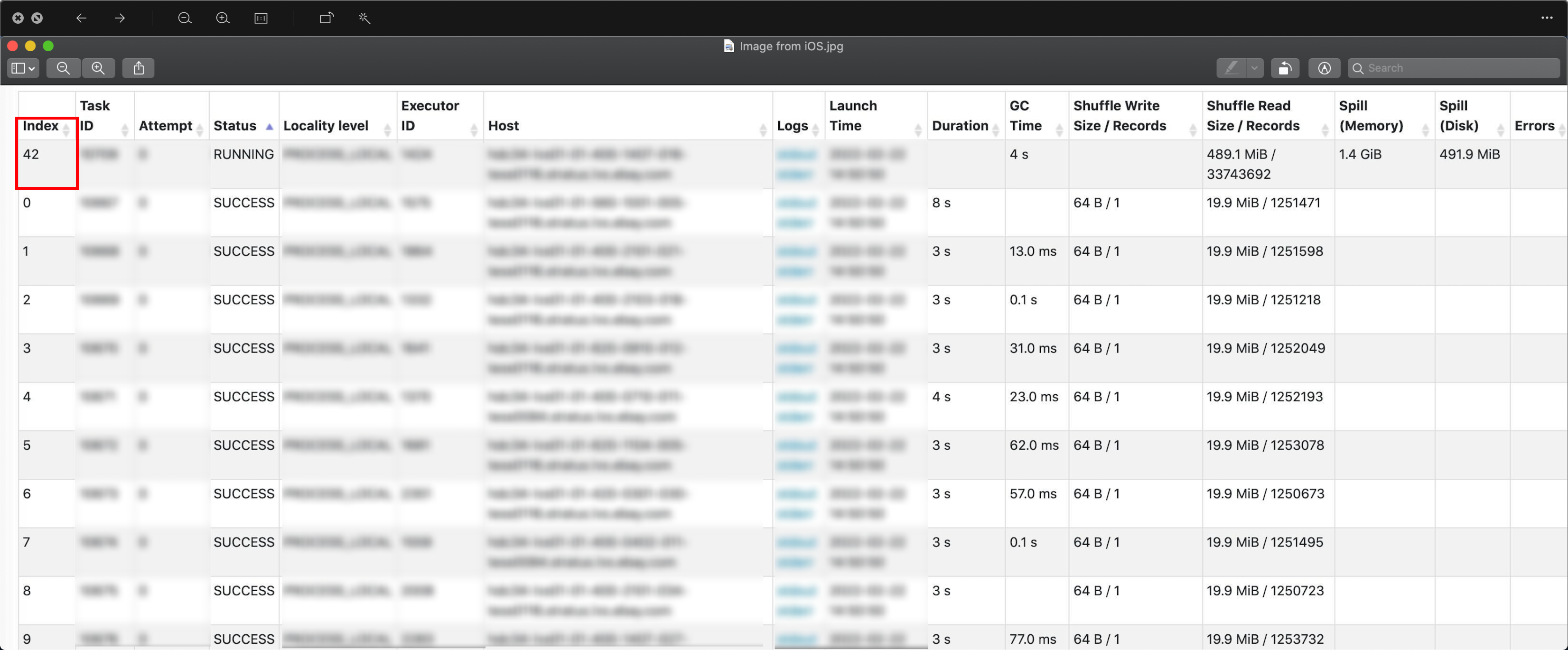
- 根据Spark task的具体执行情况来检查数据是否倾斜,从图上可以看出,其他的task都消费了19.9MB的数据,而42th task则消费了489MB的数据,任务结束的时候,实际上它消费了42GB的数据。
那么42th task都会消费到哪些数据?如何确定哪些user_id是数据倾斜呢?
- 根据Saprk的执行计划,我们发现它的join key 就是一个hash join,并且很不幸的是存在一个隐式转换,两个user_id都会被转换成double类型。
+- SortMergeJoin [knownfloatingpointnormalized(normalizenanandzero(cast(user_id#438 as double)))], [knownfloatingpointnormalized(normalizenanandzero(cast(user_id#461 as double)))], LeftOuter
注:完整的执行计划不方便看,其实就看这一行就可以。
select pmod(hash(cast (user_id as double)) ,1000) user_id,count(1) cnt
from b
group by pmod(hash(cast (user_id as double)) ,1000)
order by 2 desc;
这是所有task处理数据数量排行的前10个,可以看出42th task是其他分区的1000x。
| user_id | cnt |
|---|---|
| 42 | 2296236352 |
| 776 | 1258887 |
| 329 | 1258619 |
| 801 | 1257700 |
| 104 | 1257064 |
| 665 | 1256650 |
| 340 | 1256519 |
| 646 | 1256116 |
| 441 | 1256079 |
| 865 | 1256069 |
select user_id
from b
where pmod(hash(cast (user_id as double)) ,1000) = 42
可以看出,第42个task处理的数据全都是Nul和非数值强制转换失败认为是Null的值,以及数值的哈希码是42的。
| user_id |
|---|
| NULL |
| NULL |
| NULL |
| 05-05608-04744 |
| NULL |
| NULL |
| NULL |
| NULL |
| NULL |
| 16-05607-45983 |
| NULL |
| NULL |
| NULL |
因此,SQL的优化方式如下,我们可以对b表进行提前过滤,将其转换成decimal,并将转换失败的进行过滤。并且,你需要时刻注意链接键的数据类型是否一致。
select
    *
from a
left join (select * from b where cast(user_id as decimal) is not null) b
on a.user_id = b.user_id;
注意
一个阶段的索引等于连接键的哈希码。
pmod(hash(joinKey1 [, joinKey2, joinKey3...]) ,${partitionNumber}) = ${taskIndex}
通常partitionNumber的个数都会是1000,肯定大于42,如果分区的个数小于42时,将会是 42%partitionNumber 这个task。
所以,为什么是42?为什么Null值会放在第42个task中处理,你以为这一切都是巧合?
Spark 源码:

因此,如果你在第42个task中发现了大量的数据造成的数据倾斜,那一定是Null值引起的。
Case 3: 小表join 大表
通常,大表Left Join小表是很容易优化的,可以直接使用Map join,然而当一张小表join一张大表时,就不能用map join了。
我们来看下面这个SQL:
select
    a.user_id,
    b.risk_eval_id
from
    dw_tables.user_info_fact a
left join
    dw_tables.risk_eval_detail b
on a.user_id = b.user_id;
查看上述query的执行计划:
select
    /*+ mapjoin(b) */
    a.user_id,
    b.risk_eval_id
from
    dw_tables.user_info_fact a
left join
    dw_tables.risk_eval_detail b
on a.user_id = b.user_id;
== Physical Plan ==
AdaptiveSparkPlan isFinalPlan=false
+- Project [user_id#336, risk_eval_id#772]
+- SortMergeJoin [user_id#336], [user_id#773], LeftOuter
:- Sort [user_id#336 ASC NULLS FIRST], false, 0
: +- Exchange hashpartitioning(user_id#336, 2000), ENSURE_REQUIREMENTS, [id=#864]
: +- FileScan parquet dw_tables.user_info_fact[user_id#336] Batched: true, DataFilters: [], Format: Parquet, Location: InMemoryFileIndex[hdfs:..., PartitionFilters: [], PushedFilters: [], ReadSchema: struct<user_id:decimal(18,0)>
+- Sort [user_id#773 ASC NULLS FIRST], false, 0
+- Exchange hashpartitioning(user_id#773, 2000), ENSURE_REQUIREMENTS, [id=#857]
+- Filter isnotnull(user_id#773)
+- FileScan parquet dw_tables.risk_eval_detail[risk_eval_id#772,user_id#773] Batched: true, DataFilters: [isnotnull(user_id#773)], Format: Parquet, Location: InMemoryFileIndex[hdfs:..., PartitionFilters: [], PushedFilters: [IsNotNull(user_id)], ReadSchema: struct<risk_eval_id:decimal(18,0),user_id:decimal(18,0)>
这个SQL中,a表是一个小表,而b表是一个大表,看一下这个querry的执行计划就会发现,这只是一个普通的左链接查询.而通常,我们进行大小表join的时候,会进行Map join,小表left join 大表是可用的,而大表left join 小表就不可用了,这就会导致效率变低,任务的执行速度变慢。那我们该怎么样进行优化呢?
优化方案:虽然我们在左链接(left join)中不能对右表进行map join,但是我们仍然可以把左表推到右表。
Optimize SQL:
select
    a.user_id,
    b.risk_eval_id
from
    dw_tables.user_info_fact a
left join
    (select
        l.user_id,
        l.risk_eval_id
    from
        dw_tables.risk_eval_detail l
    semi join
        dw_tables.user_info_fact r
    on l.user_id = r.user_id)b
on a.user_id = b.user_id;
这样优化有什么好处呢? 我们来看一下优化后的执行计划,具体看一下两个query执行计划的差别。
explain
select
    a.user_id,
    b.risk_eval_id
from
    dw_tables.user_info_fact a
left join
    (select
        l.user_id,
        l.risk_eval_id
    from
        dw_tables.risk_eval_detail l
    semi join
        dw_tables.user_info_fact r
    on l.user_id = r.user_id)b
on a.user_id = b.user_id;
== Physical Plan ==
AdaptiveSparkPlan isFinalPlan=false
+- Project [user_id#336, risk_eval_id#910]
+- SortMergeJoin [user_id#336], [user_id#911], LeftOuter
:- Sort [user_id#336 ASC NULLS FIRST], false, 0
: +- Exchange hashpartitioning(user_id#336, 2000), ENSURE_REQUIREMENTS, [id=#980]
: +- FileScan parquet dw_tables.user_info_fact[user_id#336] Batched: true, DataFilters: [], Format: Parquet, Location: InMemoryFileIndex[hdfs:..., PartitionFilters: [], PushedFilters: [], ReadSchema: struct<user_id:decimal(18,0)>
+- Sort [user_id#911 ASC NULLS FIRST], false, 0
+- Exchange hashpartitioning(user_id#911, 2000), ENSURE_REQUIREMENTS, [id=#973]
+- BroadcastHashJoin [user_id#911], [user_id#336], LeftSemi, BuildRight, false
:- Filter isnotnull(user_id#911)
: +- FileScan parquet dw_tables.risk_eval_detail[risk_eval_id#910,user_id#911] Batched: true, DataFilters: [isnotnull(user_id#911)], Format: Parquet, Location: InMemoryFileIndex[hdfs:..., PartitionFilters: [], PushedFilters: [IsNotNull(user_id)], ReadSchema: struct<risk_eval_id:decimal(18,0),user_id:decimal(18,0)>
+- BroadcastExchange HashedRelationBroadcastMode(List(input[0, decimal(18,0), false]),false), [id=#969]
+- Filter isnotnull(user_id#336)
+- FileScan parquet dw_tables.user_info_fact[user_id#336] Batched: true, DataFilters: [isnotnull(user_id#336)], Format: Parquet, Location: InMemoryFileIndex[hdfs:..., PartitionFilters: [], PushedFilters: [IsNotNull(user_id)], ReadSchema: struct<user_id:decimal(18,0)>, SelectedBucketsCount: 100 out of 100
对比两个query的执行计划,不难发现优化后的执行计划,我们通过左表对右表进行过滤,这将会减小shuffle的大小,从而提高任务的执行效率。
Here is a sample of semi join
Gernal join:
with tmp1 as (
select '1' as id,'val1' as val union all
select '1' as id,'val2' as val union all
select '2' as id,'val3' as val union all
select '3' as id,'val4' as val union all
select '4' as id,'val5' as val union all
select '4' as id,'val6' as val ),
tmp2 as (
select '1' as id,'col1' as col union all
select '1' as id,'col2' as col union all
select '2' as id,'col3' as col union all
select '5' as id,'col4' as col)
select * from tmp1 a join tmp2 b on a.id = b.id
| id | val | id | col |
|---|---|---|---|
| 2 | val3 | 2 | col3 |
| 1 | val2 | 1 | col2 |
| 1 | val2 | 1 | col1 |
| 1 | val1 | 1 | col2 |
| 1 | val1 | 1 | col1 |
Semi join:
with tmp1 as (
select '1' as id,'val1' as val union all
select '1' as id,'val2' as val union all
select '2' as id,'val3' as val union all
select '3' as id,'val4' as val union all
select '4' as id,'val5' as val union all
select '4' as id,'val6' as val ),
tmp2 as (
select '1' as id,'col1' as col union all
select '1' as id,'col2' as col union all
select '2' as id,'col3' as col union all
select '5' as id,'col4' as col)
select * from tmp1 a semi join tmp2 b on a.id = b.id
| id | val |
|---|---|
| 1 | val1 |
| 1 | val2 |
| 2 | val3 |
Case 4: Cache Bucket表导致任务运行效率降低
Background:我的同事跑了一个简单的Querry查询,但是整个任务的运行非常的缓慢,于是我们对他的SQL进行了一些Check,最终发现导致任务跑的很慢的原因是由于Cache引起的。当一个临时视图在不同的SQL部分中被多次重用时,缓存这张表非常有用。但是由于Cache了一张bucket从而造成整个任务的运行都很慢。
首先,我们看一下当时的部分querry。
create or replace temproary view user_rule_actn_w as
select
    user_id,
    item_id,
    trans_id,
    pid,
    crt_dt,
    mod_dt,
    ...
from dw_tables.user_rule_actn
where
    crt_dt >= '$run_dt'
;

cache user_rule_actn_w;
这个Sql切片看起来是一个非常简单且通用的操作,但是它跑的非常慢,大概花了45min,而且它相应的task的一些指标看起来非常的奇怪。
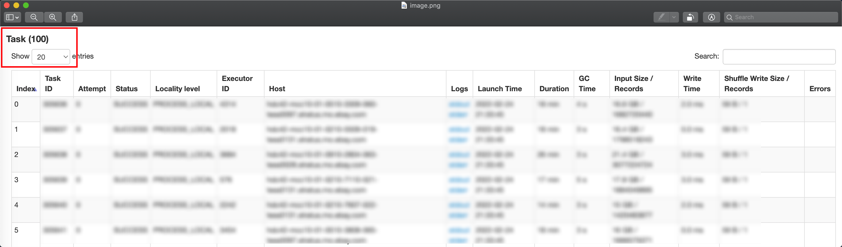
从上面有关task指标的明细中我们可以看到这个任务的并行度只有100。我们都知道没有shuffle的SQL只包含map stage, 而map的并行度可以是spark.dynamicAllocation.maxExecutors,而不是100。于是我们看了这个表的schema,发现它是一张分桶表,而它桶的个数就是100。而造成这样的原因是spark 3.2之前但凡用到了bucket表就默认会用buckets的个数作为task的个数来读数据,数据量很大的时候会很慢,只要用到分桶健,task的个数就被bucket限制。
优化方式:针对这种情况,我们的解决方案是先将分桶表中的数据读出来并插入到一张working表中,之后在根据这张working表去创建一张view,然后再对这个view进行cache,这样就不会对一张bucket表进行cache,这样task的个数就不会受到桶数量的限制。
当然,Cache的作用不仅如此,cache的时候,spark除了会将数据加载到内存落地外,还会统计数据信息,方便后面走map join。本质上是将SortMergeJoin转换成BroadcastJoin。
Case 5: 避免无意义的group by 造成的shuffle
通常,我们总是需要对一些join之后对表进行去重,这是一个很常见的操作。下面这个例子就是一个对join之后对结果进行去重的样例。
首先,我们先介绍一下常见对数据去重的方式,常用的大概有三种:
- group by:速度快,效率高,通常会sort并提前过滤。当数据量大的时候可能会慢,但慢点原因不是因为groub by,而是因为group by会在本地先sort过滤,然后再shuffle过滤,而shuffle 势必会增加运行时间。
- rownumber:会shuffle全局排序,相比group by效率就没有那么高了,但是方便业务理解。
- distinct:和group by差不多,但是不需要进行排序,数据量大时,比group by效率高,通常用来做count distinct计数。
优化案例:
select
    a.user_id,
    b.order_id,
    trans_id,
    item_id,
    ...
from
    dw_tables.user_info a
join
    dw_tables.order_info b
on a.order_id = b.order_id
group by 1,2;
从上面的SQL来看,这是一条很正常的query,拿用户表和订单表进行关联,取到每个用户相关的订单信息,然后对关联之后对数据进行一个去重,这没有什么问题,但是从业务上来说,如果你知道,用户表的user_id和订单表的order_id分别是这两个表的primary key,当我们对这两个表进行PK join的时候,并不肯能出现重复的user_id,order_id。当我们再对他进行group by的时候实际上并没有什么意义的,反而我们使用了group by就会有shuffle,这势必会增加任务的运行时间,从而降低任务的执行效率。
优化方式:在我们了解业务的前提下,要避免无意义的group by而引入的shuffle过程。
select
    a.user_id,
    b.order_id,
    trans_id,
    item_id,
    ...
from
    dw_tables.user_info a
join
    dw_tables.order_info b
on a.order_id = b.order_id
;
Case 6: Where条件与left jion时on条件的转换
想必大家都会遇到这样一种情况,在两个表join之后,where 条件中的过滤字段是否与链接条件on中的字段等价,以及二者是否可以互换位置等。对于inner join应该没有太多的异议,筛选条件放在where中还是on中情况是一样的,我们只要针对left join来说明。
网上有一种说法是这样的:
A表left join B表 on里面对B表进行过滤的条件可以放到where中, 而A表left join B表on里面对A表进行过滤的条件不可以放到where中。为什么用红色字体标注,因为这是错的,注意这是错的,错的!!!
Sample data:
create or replace temporary view user_info as(
select '1' as user_id,'1' as order_id union all
select '2' as user_id,'1' as order_id union all
select '3' as user_id,'2' as order_id union all
select '4' as user_id,'2' as order_id);

create or replace temporary view order_info as(
select '1' as order_id, 'aaa' as order_info_detail union all
select '2' as order_id, 'bbb' as order_info_detail union all
select '3' as order_id, 'ccc' as order_info_detail union all
select '4' as order_id, 'ddd' as order_info_detail );
USER_INFO:
| user_id | order_id |
|---|---|
| 1 | 1 |
| 2 | 1 |
| 3 | 2 |
| 4 | 2 |
ORDER_INFO:
| oder_id | order_info_detail |
|---|---|
| 1 | aaa |
| 2 | bbb |
| 3 | ccc |
| 4 | ddd |
Left join:
select
    a.user_id,
    a.order_id,
    b.order_info_detail
from
    user_info a,
left join
    order_info b
on
    a.order_id = b.order_id
;
| user_id | order_id | order_info_detail |
|---|---|---|
| 1 | 1 | aaa |
| 2 | 1 | aaa |
| 3 | 2 | bbb |
| 4 | 2 | bbb |
Left join on + and b表过滤条件:
select
   a.user_id,
   a.order_id,
   b.order_info_detail
from
   user_info a
left join
   order_info b
on
   a.order_id = b.order_id and b.order_id = 2;
| user_id | order_id | order_info_detail |
|---|---|---|
| 1 | 1 | null |
| 2 | 1 | null |
| 3 | 2 | bbb |
| 4 | 2 | bbb |
Left join + where b表过滤条件:
select
    a.user_id,
    a.order_id,
    b.order_info_detail
from
    user_info a
left join
    order_info b
on
    a.order_id = b.order_id
where
	b.order_id = 2;
| user_id | order_i | order_info_detail |
|---|---|---|
| 3 | 2 | bbb |
| 4 | 2 | bbb |
Left join on + and a表过滤条件:
select
    a.user_id,
    a.order_id,
    b.order_info_detail
from
    user_info a
left join
    order_info b
on
    a.order_id = b.order_id and a.user_id = 2;
| user_id | order_id | order_info_detail |
|---|---|---|
| 1 | 1 | null |
| 2 | 1 | aaa |
| 3 | 2 | null |
| 4 | 2 | null |
select
    a.user_id,
    a.order_id,
    b.order_info_detail
from
    user_info a
left join
    order_info b
on
    a.order_id = b.order_id and a.order_id = 2;
| user_id | order_id | order_info_detail |
|---|---|---|
| 1 | 1 | null |
| 2 | 1 | null |
| 3 | 2 | bbb |
| 4 | 2 | bbb |
Left join + where a表过滤条件:
select
    a.user_id,
    a.order_id,
    b.order_info_detail
from
    user_info a
left join
    order_info b
on
    a.order_id = b.order_id
where
	a.order_id = 2;
| user_id | order_i | order_info_detail |
|---|---|---|
| 3 | 2 | bbb |
| 4 | 2 | bbb |
select
    a.user_id,
    a.order_id,
    b.order_info_detail
from
    user_info a
left join
    order_info b
on
    a.order_id = b.order_id
where
	a.user_id = 2;
| user_id | order_i | order_info_detail |
|---|---|---|
| 2 | 1 | aaa |
总结:
写在on 里面的过滤条件无论是针对A表还是B表,始终都还是标准的LeftJoin,过滤条件只会影响b表的NULL值,join上就有值,join不上就是Null,并不会影响最终的结果行数,而最终结果的行数始终只与左表保持一致。而在left join后的where条件,实际上是针对left join之后形成的中间表再进行where过滤,会筛选掉不满足需求的记录(不分A表B表),因此on条件中无论针对A表过滤还是B都不可以放在where条件中。
Case 7: 避免where in中使用子查询
通常,在where中使用in本身就是很慢的,如果in条件中再使用了复杂的子查询或带有shuffle的子查询,这回大大增加任务的运行时间,效率非常低
优化案例:
select
    col1,
    col2,
    col3,
    ...
    src_last_mdfd_dt
from
    dw_tables.vender_info_data
where
    src_last_mdfd_dt in (select last_mdfd_dt from dw_tables.vender_info_data_w group by 1);
这是一个很普通的query,但是由于在in条件中使用了含shuffle的子查询导致了任务运行时间过长,效率很低的情况,通常in条件过滤的情况通常是将in转换成过滤字段>过滤条件 and 过滤字段 >过滤条件不等式的样子。
例如:
select
    col1,
    col2,
    col3,
    ...
    src_last_mdfd_dt
from
    dw_tables.vender_info_data
where
    src_last_mdfd_dt > (select min(last_mdfd_dt) from dw_tables.vender_info_data_w)
and
    src_last_mdfd_dt < (select max(last_mdfd_dt) from dw_tables.vender_info_data_w )
;
这样看似没有什么问题,但是如果last_mdfd_dt本身是不连续的情况下,会使数据量变多,这是有问题的。
优化方式:
select
    col1,
    col2,
    col3,
    ...
    src_last_mdfd_dt
from
    dw_tables.vender_info_data a
join
    dw_tables.vender_info_data_w b
on
    a.src_last_mdfd_dt = b.last_mdfd_dt;
这样就避免了where in中使用子查询而造成任务跑的非常慢点情况。
注意:
- 在使用in或者等值过滤时,隐含条件时IS NOT NULL.
- 两表left join时链接条件in中有子查询会被转换成leftsemi join。