keras 学习-线性回归

园子里头看到了一些最基础的 keras 入门指导， 用一层网络，可以训练一个简单的线性回归模型。

自己学习了一下，按照教程走下来，结果不尽如人意，下面是具体的过程。

 

第一步： 生成随机数据，绘出散点图

import numpy as np
from keras.models  import Sequential
from keras.layers import Dense 
import matplotlib.pyplot as plt

# 生产随机数据
np.random.seed(123) # 指定种子，使得每次生成的随机数保持一致
x = np.linspace(-1,1,200) # 生成一个长度为 200 的 list，数值大小在 [-1,1] 之间
np.random.shuffle(x) #随机排列传入 list 
y = 0.5 * x + 2 + np.random.normal(0, 0.05, (200,)) # 添加正态分布的偏差值

#测试数据 与 训练数据
x_train, y_train = x[:160], y[:160]
x_test, y_test = x[160:], y[160:0]

#绘出散点图: plt.scatter(x,y) plt.show()

散点图如下：

 

 二、创建网络模型

# 创建模型
model = Sequential()
# 添加全连接层,输入维度 1， 输出维度 1 
model.add(Dense(output_dim = 1, input_dim= 1))

 

三、模型编译

# 模型编译
# 损失函数：二次方的误差， 优化器：随机梯度随机梯度下降，stochastic gradient descent
model.compile(loss='mse', optimizer='sgd')  

 

四、模型训练

# 训练模型，就跑一次

print('start train model:')
for step in range(300):
    cost = model.train_on_batch(x_train, y_train)
    if step % 50 == 0:
        print('cost:', cost)

 

五、测试模型

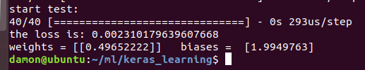
#看测试数据损失又多少
print('start test:')
cost = model.evaluate(x_test, y_test, batch_size=40)
print('the loss is:', cost)

# 查看函数参数
w,b = model.layers[0].get_weights()
print('weights =',w, '  biases = ', b)

# 用模型预测测试值
y_pred = model.predict(x_test)

# 画出测试散点图
plt.scatter(x_test, y_test)
# 画出回归线
plt.plot(x_test, y_pred)
plt.show()

     输出结果： 

 

 

此次训练所得模型：

 

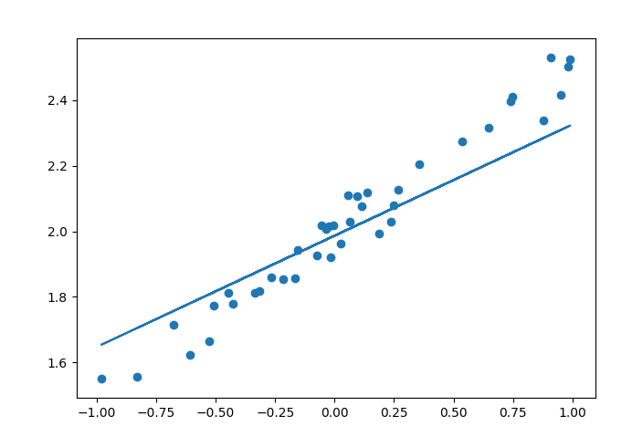
从图中可以看出，模型没有很好的满足我们的需求，进行调整，看下结果：

减小batch_size, 增加训练次数。

batch_size: 单一批训练样本数量

epochs : 将全部样本训练都跑一遍为 1 个 epoch,  10 个 epochs 就是全部样本都训练 10 次

# 调整模型训练过程
model.fit(x_train, y_train, batch_size=5,epochs=60)

 

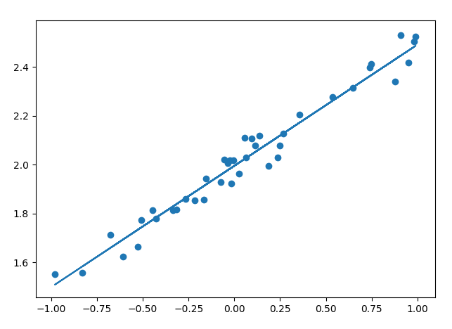
最终所得模型图为：

 

 曲线为：