【论文阅读】DSTAGNN Dynamic Spatial-Temporal Aware Graph Neural Network for Traffic Flow Forecasting
DSTAGNN Dynamic Spatial-Temporal Aware Graph Neural Network for Traffic Flow Forecasting
Info
- title: DSTAGNN: Dynamic Spatial-Temporal Aware Graph Neural Network for Traffic Flow Forecasting
- publish: ICML 2022
- url: dblp: DSTAGNN: Dynamic Spatial-Temporal Aware Graph Neural Network for Traffic Flow Forecasting. (uni-trier.de)
- corresponding author: ShiYong Lan
- first author:
- ShiYong Lan
- Yitong Ma
Model
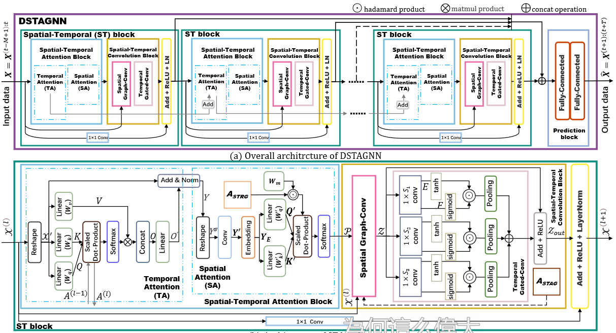
Network Structure
Details
0. 前置知识
节点:
节点数量:
节点间连接(边):
图:
邻接矩阵:
t时刻的图信号:
数据记录:
预测目标:
模型
1. 节点特征的表示与转换
Take the traffic flow
at the N recording points for D days as an example, where dt is the number of recording times per day (if recordings are taken once every 5 minutes, then = 288).
For each recording point, the oneday traffic data is treated as a vector, then a set of multi-day traffic data is denoted as a vector sequence. For example, the vector sequence obtained at recording point n () is denoted as , , where .
提取交通流量信息:
In this way, the vector sequence of the recording point n is transformed into a probability distribution
, and each day has a probability mass and , which denotes the proportion of traffic volume in a certain day over a period of time.
P.S.
- 为什么流量信息是一天的流量占一段时间的比?
- 这里为什么用二范数,而不是直接对一天各个时段的流量进行求和?
2. 时空感知距离与时空关联图
概率分布变换代价(使用Wassertein距离):
利用余弦距离作为变换代价:
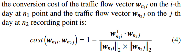
使用Wassertein距离计算两个节点的差异:
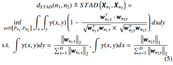
节点间的关联度矩阵
通过设定稀疏水平
对时空关联图
P.S.
- 为什么用余弦变换作为代价?
- 为什么用Wassertein距离计算节点的差异(关联)?
- 为什么关联图中只选了
3. 时空注意力块
这里用到了多头注意力机制,参考Attention Is All You Need。
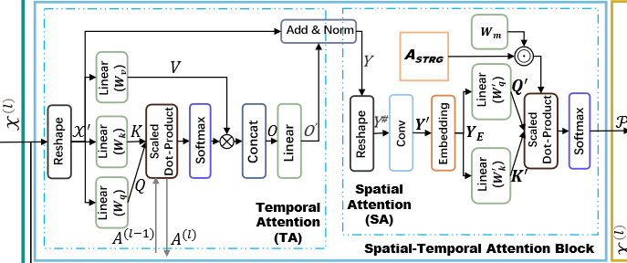
时间注意力
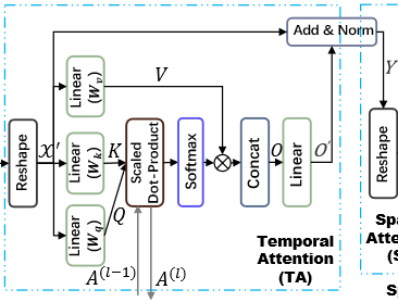
- 这里的
- 注意力*:
- Scaled Dot-Product(论文Attention Is All You Need里来的。)
- 注意力:
- Scaled Dot-Product(论文Attention Is All You Need里来的。)
- 多头注意力机制(论文Attention Is All You Need里来的。)
- Concat:
- Linear层把输出的大小还原,获得
- 带残差的LayerNorm:
P.S. - 原文中的LayerNorm公式错了。
- Scaled Dot-product 为什么用残差?
空间注意力
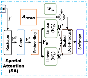
- Reshape:
- Conv:
- 先把
- 对特征维
- Embedding:
Then, we add positional information to
- 先把
- 注意力机制(这里的空间注意力其实只算了注意力中的相关性,在下一步卷积中使用):
Instead of using the self-attention fully generated from
P.S.
- Conv中的高维映射怎么映射?为什么要映射?
- Conv中的一维卷积怎么把整个
- 这里为什么不用残差了,而是用
4. Spatial-Temporal Convolution Block
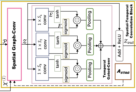
空间图卷积
这里使用了ChebyNet卷积,待深入。
图信号:
归一化的拉普拉斯矩阵:
邻接矩阵:
参数:
第k个头的空间-时间注意力矩阵:
P.S.
- 为什么把P直接哈达玛乘在切比雪夫多项式上?
时间门控卷积(Temporal gated convolution)
论文提出了M-GTU (Multi-scale Gated Tanh Unit) 卷积模块捕捉交通流数据中的动态时间信息。
M-GTU由三个GTU模块组成,每个GTU由Convolution和Gating两步组成。
- 卷积:
- 输入:
- 卷积核:
- 卷积公式:
- 输入:
- Gating:把
- Concat:虽然图上有Pooling,但是代码中并没有,使用三个不同的卷积核
- Linear:将Concat的结果放进Linear层,恢复原来的大小。
self.fcmy = nn.Sequential(
    nn.Linear(3 * num_of_timesteps - 12, num_of_timesteps),
    nn.Dropout(0.05),
)
P.S.
- 为什么要用GTU?
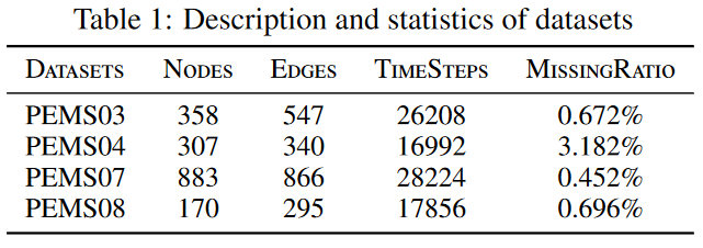
Datasets
文章使用了PEMS03、PEMS04、PEMS07、PEMS08三个数据集。


【推荐】国内首个AI IDE,深度理解中文开发场景,立即下载体验Trae
【推荐】编程新体验,更懂你的AI,立即体验豆包MarsCode编程助手
【推荐】抖音旗下AI助手豆包,你的智能百科全书,全免费不限次数
【推荐】轻量又高性能的 SSH 工具 IShell:AI 加持,快人一步
· 震惊!C++程序真的从main开始吗?99%的程序员都答错了
· 别再用vector<bool>了!Google高级工程师:这可能是STL最大的设计失误
· 单元测试从入门到精通
· 【硬核科普】Trae如何「偷看」你的代码?零基础破解AI编程运行原理
· 上周热点回顾(3.3-3.9)