再读目标检测--ssd深度解析
[目标检测 -- R-CNN,Fast R-CNN,Faster R-CNN] https://www.cnblogs.com/yanghailin/p/14767995.html
[目标检测---SSD] https://www.cnblogs.com/yanghailin/p/14769384.html
[ssd 的anchor生成详解] https://www.cnblogs.com/yanghailin/p/14868575.html
[ssd 网络详解] https://www.cnblogs.com/yanghailin/p/14871296.html
[ssd loss详解] https://www.cnblogs.com/yanghailin/p/14882807.html
其实前阵子读过ssd源码,并且也写出了上面的博客,然后再隔一阵子我就完全不记得了。。。然后最近又再读了一下,但是这次读源码的速度明显快多了,
特别是一些之前似懂非懂的地方都有进一步理解了。
ssd网络部分
我又手写了一遍。。。
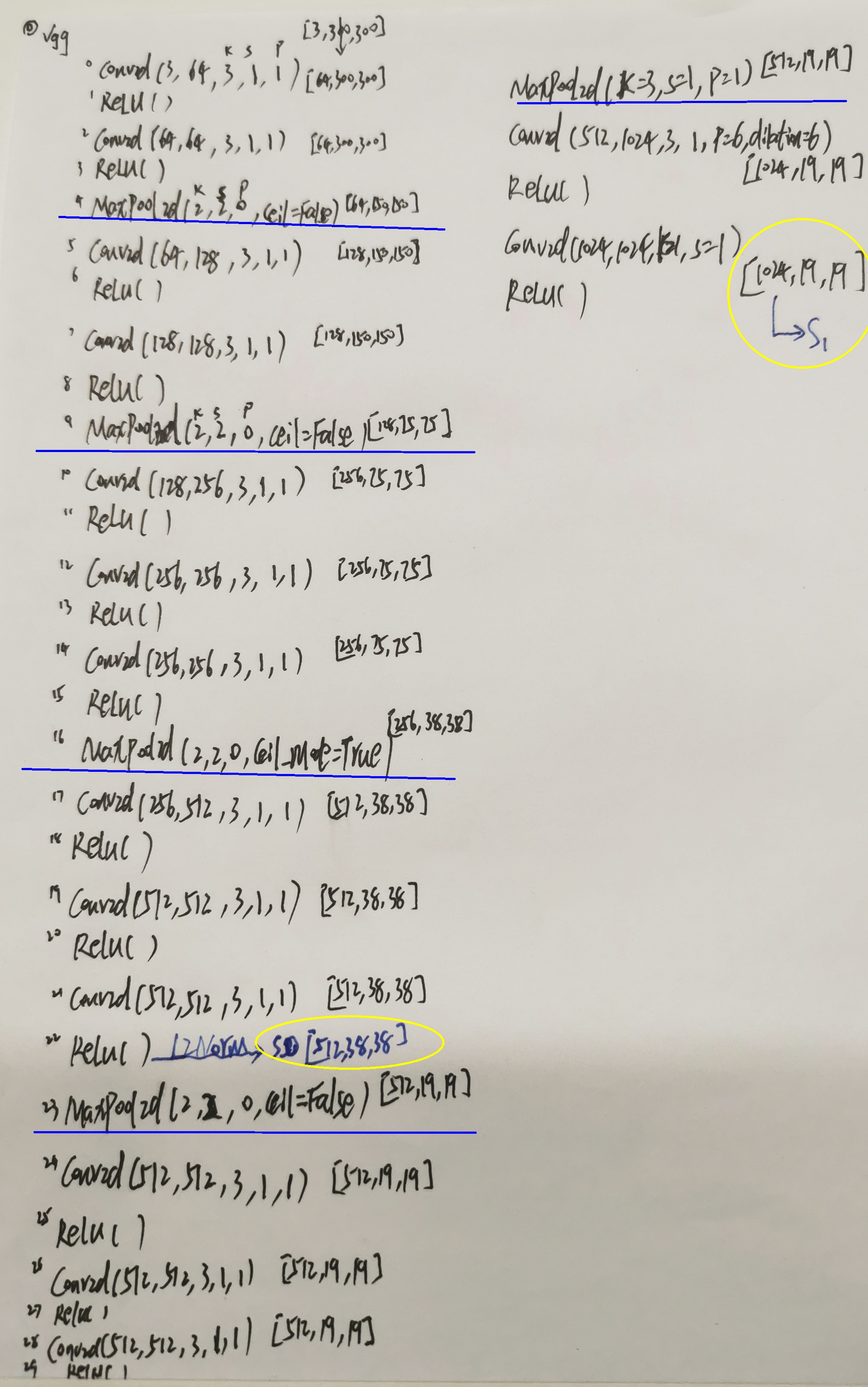
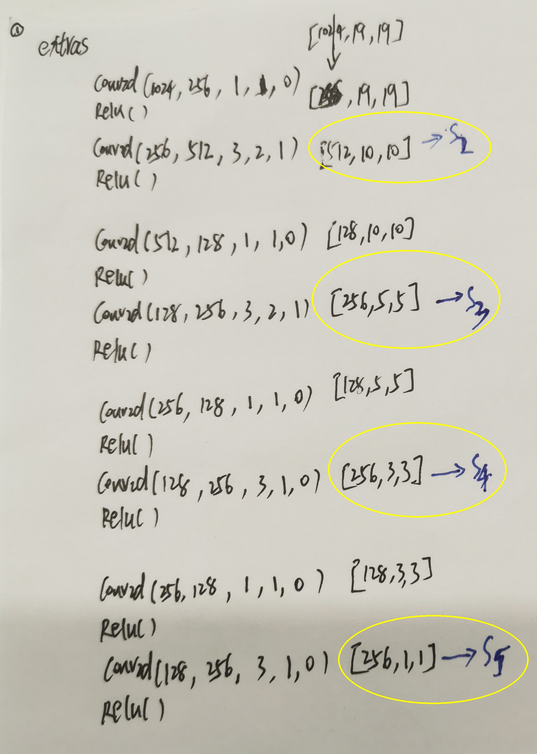
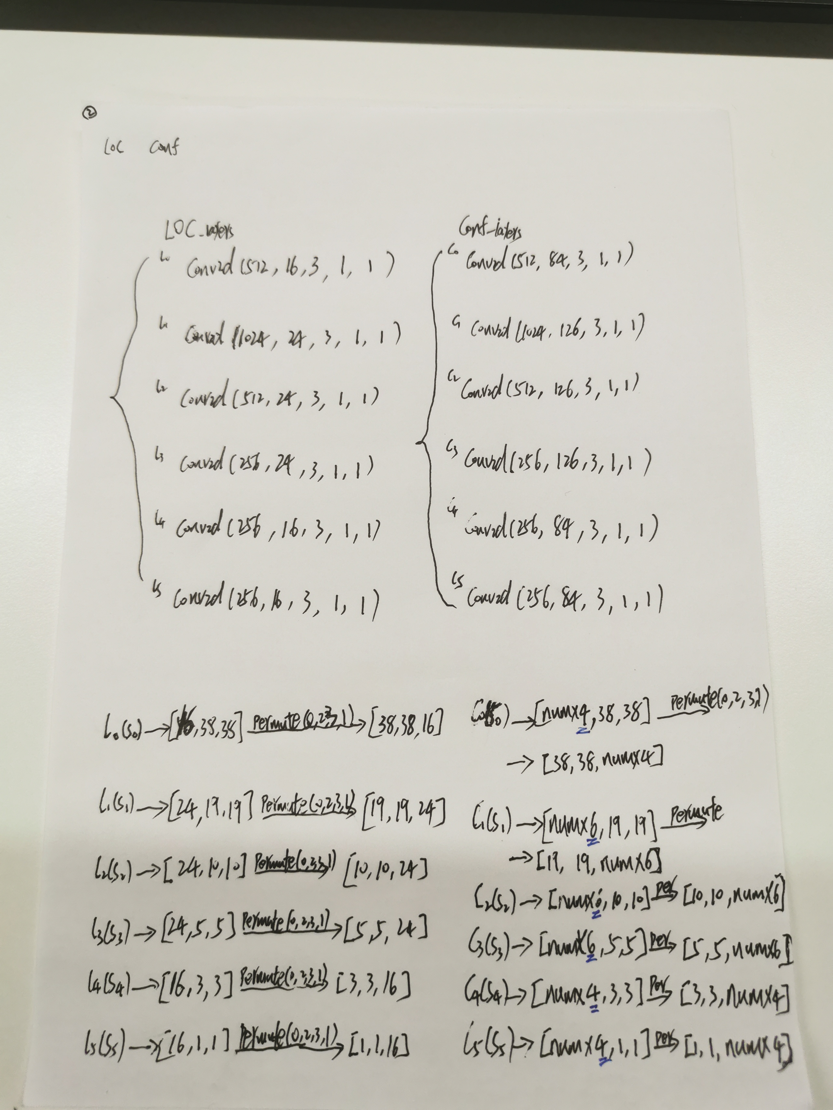
上面我根据代码写的图就和论文中这个图一致:
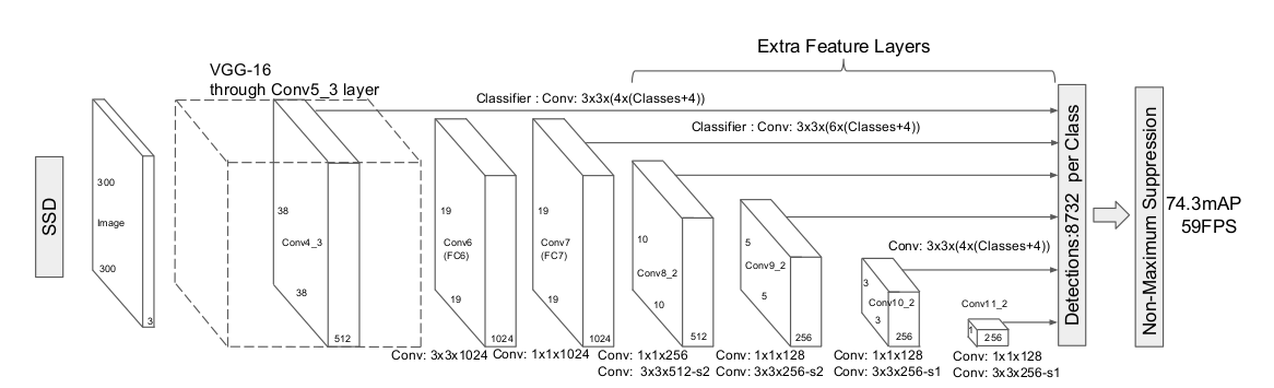
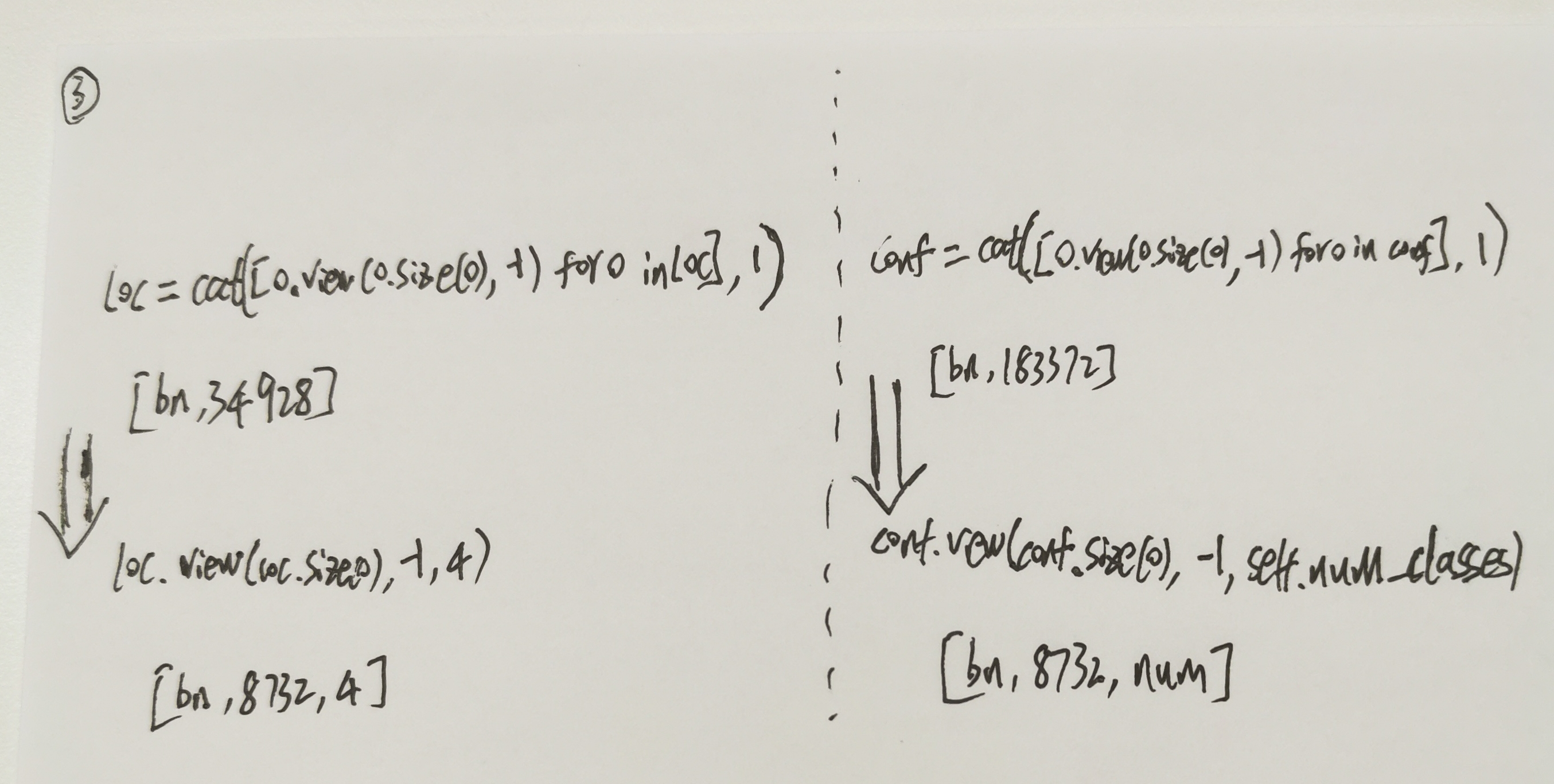
我上面最后的LOC [bn,8732,4]
conf [bn,8732,num]
就是网络的输出。
ssd loss部分 -- ssd编解码
关于编解码,我一开始看的时候也是看的稀里糊涂的,你说这么整就这样呗。ssd论文里面公式就是如下:
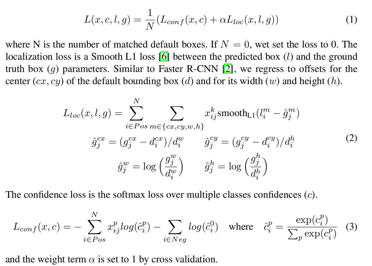
然后我看到faster rcnn里面有详细的介绍。
https://blog.csdn.net/weixin_42782150/article/details/110522380
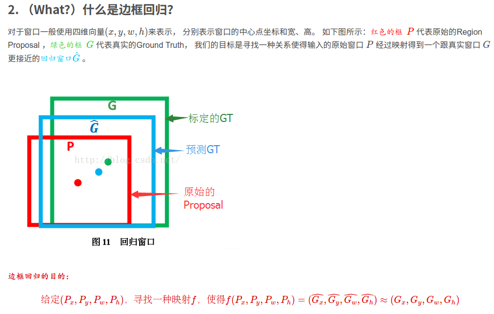
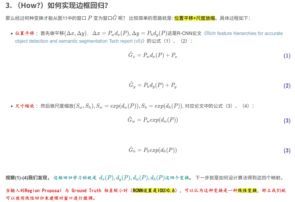
预测的框为了和gt靠拢,需要把anchor框中心点x,y加上一个偏移量,宽高乘以一个系数不为0系数!向gt靠拢,所以产生了这种数学公式。

在faster rcnn论文里面:
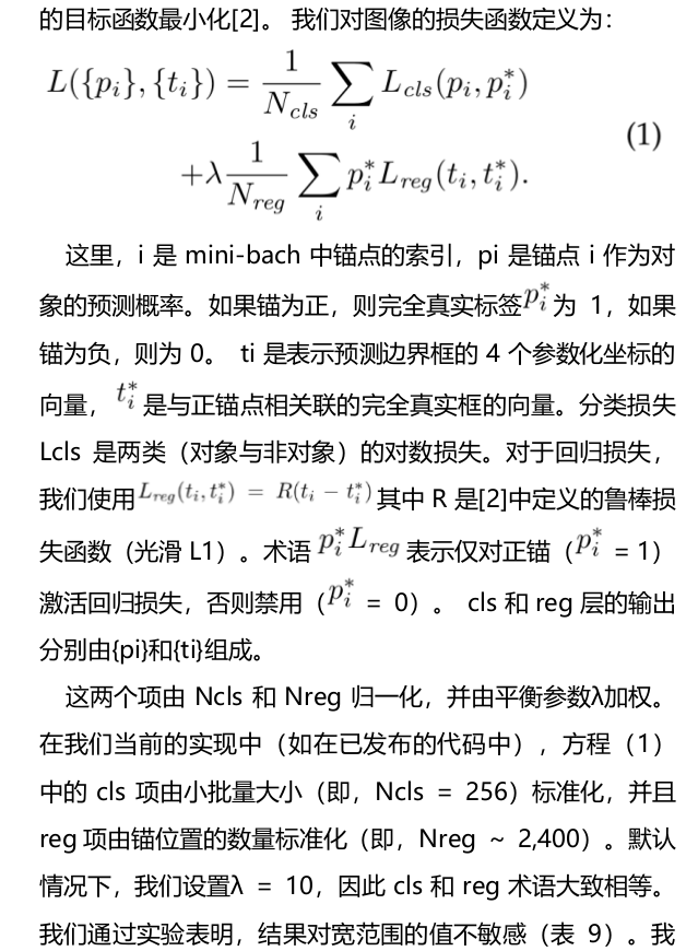
可以看到是有两组t和t.
一开始看看不懂,后来荒原大悟!
下面的t公式是gt与anchor之间的偏移。而网络学习就是学习的这种偏移t!看上面loss的公式,就是t和t。为了就是让网络向t靠拢。
t就是编码之后的,这种编码关系就是如上式所示。
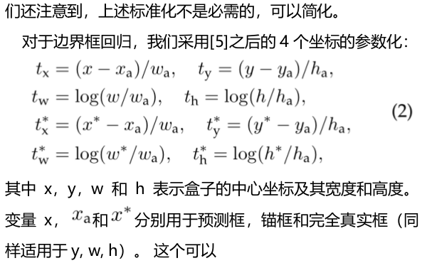
关于如何算交并比,没看到映射到原图的操作。
计算交并比,没有看到一处for循环。
def point_form(boxes):
    """ Convert prior_boxes to (xmin, ymin, xmax, ymax)
    representation for comparison to point form ground truth data.
    Args:
        boxes: (tensor) center-size default boxes from priorbox layers.
    Return:
        boxes: (tensor) Converted xmin, ymin, xmax, ymax form of boxes.
    """
    return torch.cat((boxes[:, :2] - boxes[:, 2:]/2,     # xmin, ymin
                     boxes[:, :2] + boxes[:, 2:]/2), 1)  # xmax, ymax
def intersect(box_a, box_b):
    """ We resize both tensors to [A,B,2] without new malloc:
    [A,2] -> [A,1,2] -> [A,B,2]
    [B,2] -> [1,B,2] -> [A,B,2]
    Then we compute the area of intersect between box_a and box_b.
    Args:
      box_a: (tensor) bounding boxes, Shape: [A,4].
      box_b: (tensor) bounding boxes, Shape: [B,4].
    Return:
      (tensor) intersection area, Shape: [A,B].
    """
    A = box_a.size(0)
    B = box_b.size(0)

    # n1 = box_a[:, 2:]
    # n1_1 = box_a[:, 2:].unsqueeze(1)
    # n1_2 = box_a[:, 2:].unsqueeze(1).expand(A, B, 2)
    #
    # n2 = box_b[:, 2:]
    # n2_1 = box_b[:, 2:].unsqueeze(0)
    # n2_2 = box_b[:, 2:].unsqueeze(0).expand(A, B, 2)
    #
    # n3 = torch.min(n1_2, n2_2)

    max_xy = torch.min(box_a[:, 2:].unsqueeze(1).expand(A, B, 2),
                       box_b[:, 2:].unsqueeze(0).expand(A, B, 2))
    min_xy = torch.max(box_a[:, :2].unsqueeze(1).expand(A, B, 2),
                       box_b[:, :2].unsqueeze(0).expand(A, B, 2))

    # sub_ = max_xy - min_xy

    inter = torch.clamp((max_xy - min_xy), min=0)
    return inter[:, :, 0] * inter[:, :, 1]


def jaccard(box_a, box_b):
    """Compute the jaccard overlap of two sets of boxes.  The jaccard overlap
    is simply the intersection over union of two boxes.  Here we operate on
    ground truth boxes and default boxes.
    E.g.:
        A ∩ B / A ∪ B = A ∩ B / (area(A) + area(B) - A ∩ B)
    Args:
        box_a: (tensor) Ground truth bounding boxes, Shape: [num_objects,4]
        box_b: (tensor) Prior boxes from priorbox layers, Shape: [num_priors,4]
    Return:
        jaccard overlap: (tensor) Shape: [box_a.size(0), box_b.size(0)]
    """
    inter = intersect(box_a, box_b)
    area_a = ((box_a[:, 2]-box_a[:, 0]) *
              (box_a[:, 3]-box_a[:, 1])).unsqueeze(1).expand_as(inter)  # [A,B]
    area_b = ((box_b[:, 2]-box_b[:, 0]) *
              (box_b[:, 3]-box_b[:, 1])).unsqueeze(0).expand_as(inter)  # [A,B]
    union = area_a + a
    rea_b - inter
    return inter / union  # [A,B]

overlaps = jaccard(
        truths,
        point_form(priors)
    )
看了代码,所有的操作都是相对值,0-1之间的数值。这个数值乘以原图大小就能映射到原图,所以代码中都是相对值,和在原图上操作一致。
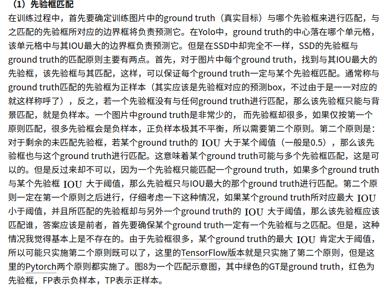
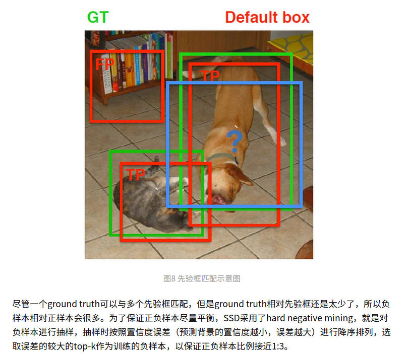
先验框匹配规则
在算gt与anchor交并比的时候。一张图的gt很少,1,2个目标,anchor有8732个。
代码中的策略是保证一个gt与最大交并比的anchor匹配,然后每个anchor匹配一个与其交并比最大的gt!
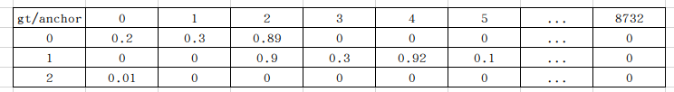
看这张图,先横向的找到gt与anchor最大的那个,这个是最大优先级且后续有逻辑确保这个始终满足。
 best_truth_overlap.index_fill_(0, best_prior_idx, 2)  # ensure best prior
    # TODO refactor: index  best_prior_idx with long tensor
    # ensure every gt matches with its prior of max overlap
    for j in range(best_prior_idx.size(0)):
        best_truth_idx[best_prior_idx[j]] = j
再纵向的找最大,就是每个anchor对应最大交并比的gt。然后把8732个anchor与匹配的gt编码。
把anchor与gt交并比小于一定阈值的置位背景类。
之前我的博客有分析:
https://www.cnblogs.com/yanghailin/p/14882807.html
这个知乎有关于先验框匹配的一段讲解:https://zhuanlan.zhihu.com/p/33544892
难例挖掘部分:
挺难的,有一段还是不理解。但是感觉设计的很巧妙!两次sort。
 #loss_c[26196,1]    #https://zhuanlan.zhihu.com/p/153535799
loss_c = log_sum_exp(batch_conf) - batch_conf.gather(1, conf_t.view(-1, 1))
这里放出我详细注释的代码
# -*- coding: utf-8 -*-
import torch
import torch.nn as nn
import torch.nn.functional as F
from torch.autograd import Variable
from data import coco as cfg
from ..box_utils import match, log_sum_exp

# criterion = MultiBoxLoss(cfg['num_classes'], 0.5, True, 0, True, 3, 0.5,
#                          False, args.cuda)

class MultiBoxLoss(nn.Module):
    """SSD Weighted Loss Function
    Compute Targets:
        1) Produce Confidence Target Indices by matching  ground truth boxes
           with (default) 'priorboxes' that have jaccard index > threshold parameter
           (default threshold: 0.5).
        2) Produce localization target by 'encoding' variance into offsets of ground
           truth boxes and their matched  'priorboxes'.
        3) Hard negative mining to filter the excessive number of negative examples
           that comes with using a large number of default bounding boxes.
           (default negative:positive ratio 3:1)
    Objective Loss:
        L(x,c,l,g) = (Lconf(x, c) + αLloc(x,l,g)) / N
        Where, Lconf is the CrossEntropy Loss and Lloc is the SmoothL1 Loss
        weighted by α which is set to 1 by cross val.
        Args:
            c: class confidences,
            l: predicted boxes,
            g: ground truth boxes
            N: number of matched default boxes
        See: https://arxiv.org/pdf/1512.02325.pdf for more details.
    """

    def __init__(self, num_classes, overlap_thresh, prior_for_matching,
                 bkg_label, neg_mining, neg_pos, neg_overlap, encode_target,
                 use_gpu=True):
        super(MultiBoxLoss, self).__init__()
        self.use_gpu = use_gpu
        self.num_classes = num_classes
        self.threshold = overlap_thresh
        self.background_label = bkg_label
        self.encode_target = encode_target
        self.use_prior_for_matching = prior_for_matching
        self.do_neg_mining = neg_mining
        self.negpos_ratio = neg_pos
        self.neg_overlap = neg_overlap
        self.variance = cfg['variance']

    def forward(self, predictions, targets):
        """Multibox Loss
        Args:
            predictions (tuple): A tuple containing loc preds, conf preds,
            and prior boxes from SSD net.
                conf shape: torch.size(batch_size,num_priors,num_classes)
                loc shape: torch.size(batch_size,num_priors,4)
                priors shape: torch.size(num_priors,4)

            targets (tensor): Ground truth boxes and labels for a batch,
                shape: [batch_size,num_objs,5] (last idx is the label).

                loc_data [3,8732,4]
                conf_data [3,8732,21]
                priors [8732,4]
        """
        loc_data, conf_data, priors = predictions
        num = loc_data.size(0) # num就是batchsize
        priors = priors[:loc_data.size(1), :] #priors [8732,4]
        num_priors = (priors.size(0)) #num_priors=8732
        num_classes = self.num_classes #21

        # match priors (default boxes) and ground truth boxes
        loc_t = torch.Tensor(num, num_priors, 4) #[3,8732,4]
        conf_t = torch.LongTensor(num, num_priors) #[3,8732]
        for idx in range(num):
            truths = targets[idx][:, :-1].data
            labels = targets[idx][:, -1].data
            defaults = priors.data
            match(self.threshold, truths, defaults, self.variance, labels,
                  loc_t, conf_t, idx)
        if self.use_gpu:
            loc_t = loc_t.cuda()
            conf_t = conf_t.cuda()

        #后缀_t的变量是代表truth
        #这里经过match出来得到的loc_t[3,8732,4], conf_t[3,8732]
        #loc_t[3,8732,4] 是每个anchor与gt做了编码之后的值
        #conf_t[3, 8732] 是label,0-21之间的值,大部分地方为0,只有anchor与gt交并比大于阈值的地方才有值
        # wrap targets
        loc_t = Variable(loc_t, requires_grad=False) #[3,8732,4]
        conf_t = Variable(conf_t, requires_grad=False) #[3,8732]

        # pos [3,8732]  False,True 重要! 挑选出正样本位置,正样本位置上是true,其余为false
        # num_pos shape[3,1]   | [23],[4],[9]   每张图正样本个数
        pos = conf_t > 0 #pos [3,8732]  False,True
        num_pos = pos.sum(dim=1, keepdim=True) #num_pos shape[3,1]   | [23],[4],[9]


        # Localization Loss (Smooth L1)
        #pos [3,8732]
        #pos.dim()=2
        #pos.unsqueeze(pos.dim()) [3,8732,1]
        # loc_data [3,8732,4]
        # pos_idx [3,8732,4] True  False   || 就是把pos里面的True和False放大到[3,8732,4]
        pos_idx = pos.unsqueeze(pos.dim()).expand_as(loc_data)

        #loc_data[3, 8732, 4]   aa[144]
        aa = loc_data[pos_idx]
        #[3,8732,4]   bb[144]
        bb = loc_t[pos_idx]

        #pos_idx [3,8732,4] True  False
        #loc_data [3,8732,4]  网络预测输出值
        #loc_data[pos_idx] shape[144]  (23+4+9)×4=144
        # loc_t [3,8732,4]
        #loc_t[pos_idx] shape[144]  (23+4+9)×4=144
        loc_p = loc_data[pos_idx].view(-1, 4)
        loc_t = loc_t[pos_idx].view(-1, 4)
        #loss_l tensor(14.0165, grad_fn=<SmoothL1LossBackward>)
        loss_l = F.smooth_l1_loss(loc_p, loc_t, size_average=False)

        # Compute max conf across batch for hard negative mining
        #conf_data [3,8732,21]  网络预测值
        # batch_conf[3*8732,21]  [26196,21]
        # tt_1 = batch_conf.max() ## 35
        # tt_2 = batch_conf.min() ## -13
        #这里取出了最大最小值方便直观的感受一下里面值都是啥,可以看到这个值其实是为了预测label的。没有经过softmax
        batch_conf = conf_data.view(-1, self.num_classes)

        b1 = log_sum_exp(batch_conf) #[26196,1]
        # conf_t[3,8732]
        # conf_t.view(-1, 1) [26196,1]
        b2 = batch_conf.gather(1, conf_t.view(-1, 1)) #[26196,1]


        #https://blog.csdn.net/liyu0611/article/details/100547145
        #https://zhuanlan.zhihu.com/p/35709485
        # https://zhuanlan.zhihu.com/p/153535799
        #loss_c[26196,1]
        loss_c = log_sum_exp(batch_conf) - batch_conf.gather(1, conf_t.view(-1, 1))

        # Hard Negative Mining
        #loss_c[pos] = 0  # filter out pos boxes for now
        #loss_c = loss_c.view(num, -1)
        #loss_c [3,8732]
        loss_c = loss_c.view(num, -1)
        #pos [3,8732]
        # loss_c [3,8732]
        loss_c[pos] = 0 #把正样本的loss置为0

        #两次sort https://blog.csdn.net/laizi_laizi/article/details/103482634
        #loss_idx [3,8732]
        tmp1, loss_idx = loss_c.sort(1, descending=True) ## _, loss_idx = loss_c.sort(1, descending=True)
        #idx_rank [3,8732]
        tmp2, idx_rank = loss_idx.sort(1) ## _, idx_rank = loss_idx.sort(1)

        # pos [3,8732]
        # num_pos shape[3,1]   | [23],[4],[9]
        num_pos = pos.long().sum(1, keepdim=True)

        # aaaaa shape[3,1]   | [23*3],[4*3],[9*3]
        #aaaaa = self.negpos_ratio * num_pos
        # num_neg shape[3,1]   | [23*3],[4*3],[9*3]
        num_neg = torch.clamp(self.negpos_ratio*num_pos, max=pos.size(1)-1)#num_pos shape[3,1]   | [69],[12],[27]

        # num_neg shape[3,1]
        # idx_rank[3,8732]
        #neg [3,8732]  True,False  给出的是loss_c对应坐标的True与False 排序的从大到小
        neg = idx_rank < num_neg.expand_as(idx_rank)
        # Confidence Loss Including Positive and Negative Examples
        # pos[3,8732]
        # pos.unsqueeze(2)  [3,8732,1]
        #conf_data[3, 8732, 21]
        #pos_idx [3, 8732, 21]
        pos_idx = pos.unsqueeze(2).expand_as(conf_data)#pos[3,8732]  conf_data[3,8732,21]
        # neg [3,8732]
        # neg_idx [3, 8732, 21]
        neg_idx = neg.unsqueeze(2).expand_as(conf_data)##neg [3,8732]  conf_data[3,8732,21]


        # tmp_1111 = pos_idx + neg_idx #[3,8732,21]  True  False   ##其他的 pos_idx+neg_idx  这两者的形状都是相同的[3,8732,21] 值都是True或者False  加运算相当执行了或运算,只要有一个True就是True
        # tmp_2222 = (pos_idx+neg_idx).gt(0) #[3,8732,21]  True  False
        # conf_data [3,8732,21]
        # tmp_333 = conf_data[(pos_idx + neg_idx).gt(0)] #[3696]
        #conf_p [176,21]          #其他的 conf_p [144,21] -->  这里面的144就是上面两个pos_idx和neg_idx里面True数量之和 69+12+27+23+4+9=144
        conf_p = conf_data[(pos_idx+neg_idx).gt(0)].view(-1, self.num_classes)
        # pos [3,8732]
        # neg [3,8732]
        # conf_t [3,8732]
        # targets_weighted  [176]   ||[144]
        targets_weighted = conf_t[(pos+neg).gt(0)]
        #loss_c tensor(58.0656, grad_fn=<NllLossBackward>)
        loss_c = F.cross_entropy(conf_p, targets_weighted, size_average=False)

        # Sum of losses: L(x,c,l,g) = (Lconf(x, c) + αLloc(x,l,g)) / N

        N = num_pos.data.sum() ##N=36  就是num_pos之和[23] + [4] + [9]
        loss_l /= N
        loss_c /= N
        return loss_l, loss_c
有两个地方需要说一下:
第一个地方就是
loss_c = log_sum_exp(batch_conf) - batch_conf.gather(1, conf_t.view(-1, 1))
这个其实感觉就是交叉熵,log_sum_exp就是下面公式后面减号部分,batch_conf.gather(1, conf_t.view(-1, 1))就是xj
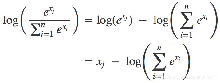
公式来源于下面博客。
https://blog.csdn.net/liyu0611/article/details/100547145
之所以要log_sum_exp,是因为e的1000次方会超数值表达范围。具体的看https://zhuanlan.zhihu.com/p/153535799
就是搞不明白如下:
loss_c = log_sum_exp(batch_conf) - batch_conf.gather(1, conf_t.view(-1, 1))
loss_c = F.cross_entropy(conf_p, targets_weighted, size_average=False)
有啥区别,为啥第一个要这么写。
还有就是两次sort
https://blog.csdn.net/laizi_laizi/article/details/103482634
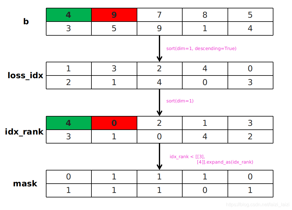
这个图片就显示的很清楚了,两次sort就是为了能够方便取出排名前多少的数值,并且得到其位置。很厉害!