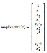
Regularized logistic regression : mapFeature(将feature增多) and costFunctionReg
ex2_reg.m文件中的部分内容
%% =========== Part 1: Regularized Logistic Regression ============
% In this part, you are given a dataset with data points that are not
% linearly separable. However, you would still like to use logistic
% regression to classify the data points.
%
% To do so, you introduce more features to use -- in particular, you add
% polynomial features to our data matrix (similar to polynomial
% regression).
%
% Add Polynomial Features
% Note that mapFeature also adds a column of ones for us, so the intercept
% term is handled
X = mapFeature(X(:,1), X(:,2)); %调用下面的mapFeature.m文件中的mapFeature(X1,X2)函数
%将只有x1,x2feature map成一个有28个feature的6次的多项式  ,这样就能画出更复杂的decision boundary, 但同时也有可能带来overfitting的结果(取决于λ的值)
% 调用完后X变为118*28(118个example,28个属性,包括前面的1做为一列)的矩阵
% Initialize fitting parameters
initial_theta = zeros(size(X, 2), 1); %initial_theta: 28*1
% Set regularization parameter lambda to 1
lambda = 1; % λ=1;当λ=0时表示不正则化(No regularization ),这时会出现overfitting;当λ=100时会出现Too much regularization(Underfitting)
% Compute and display initial cost and gradient for regularized logistic
% regression
[cost, grad] = costFunctionReg(initial_theta, X, y, lambda); %调用costFunctionReg.m文件中的costFunctionReg(theta, X, y, lambda)函数
fprintf('Cost at initial theta (zeros): %f\n', cost); %计算initial theta (zeros)时的cost 值
fprintf('\nProgram paused. Press enter to continue.\n');
pause;
mapFeature.m文件
function out = mapFeature(X1, X2)
% MAPFEATURE Feature mapping function to polynomial features
%
% MAPFEATURE(X1, X2) maps the two input features
% to quadratic features used in the regularization exercise.
%
% Returns a new feature array with more features, comprising of
% X1, X2, X1.^2, X2.^2, X1*X2, X1*X2.^2, etc..
%
% Inputs X1, X2 must be the same size
%
degree = 6; %map the features into all polynomial terms of x1 and x2 up to the sixth power
out = ones(size(X1(:,1)));
for i = 1:degree
for j = 0:i
out(:, end+1) = (X1.^(i-j)).*(X2.^j);
end
end
end
costFunctionReg.m文件
function [J, grad] = costFunctionReg(theta, X, y, lambda)
%COSTFUNCTIONREG Compute cost and gradient for logistic regression with regularization
% J = COSTFUNCTIONREG(theta, X, y, lambda) computes the cost of using
% theta as the parameter for regularized logistic regression and the
% gradient of the cost w.r.t. to the parameters.
% Initialize some useful values
m = length(y); % number of training examples
% You need to return the following variables correctly
J = 0;
grad = zeros(size(theta));
% ====================== YOUR CODE HERE ======================
% Instructions: Compute the cost of a particular choice of theta.
% You should set J to the cost.
% Compute the partial derivatives and set grad to the partial
% derivatives of the cost w.r.t. each parameter in theta
J = 1/m*(-1*y'*log(sigmoid(X*theta)) - (ones(1,m)-y')*log(ones(m,1)-sigmoid(X*theta)))...
+ lambda/(2*m) * (theta(2:end,:))' * theta(2:end,:); %Note that you should not regularize the parameter θ0.
 the regularized cost function,
grad = 1/m * (X' * (sigmoid(X*theta) - y)) + (lambda/m)*theta; % 
grad(1) = 1/m * (X(:,1))' * (sigmoid(X*theta) - y); %
% Note that you should not regularize the parameter θ0.
% =============================================================
end


 浙公网安备 33010602011771号