

近端策略优化(PPO)
背景
前面我们介绍了策略梯度算法,但是其存在两个缺点:
1. 每条采样的数据只能更新模型一次,采样数据的成本高
2. 由于没有对梯度加限制,训练不稳定,容易陷入局部最优
下面我们看一下PPO算法是如何解决这两个问题的
重要性采样
假设我们有一个函数 f(x),要计算从分布 p 采样 x,再把 x 代入 f ,得到 f(x)。我们该怎么计算 f(x) 的期望值呢? 假设我们不能对分布 p 做积分,但可以从分布 p 采样一些数据 xi。把 xi 代入 f(x),取 它的平均值,就可以近似 f(x) 的期望值:
\[ \mathbb{E}_{x \sim p} [f(x)] \approx \frac{1}{N} \sum_{i = 1}^{N} f(x^i) \]
现在有另外一个问题,假设我们不能从分布 p 采样数据,只能从另外一个分布 q 采样数据 x,q 可以是任何分布,我们对其做如下的变换:
\[ \int f(x) p(x) \mathrm{d}x = \int f(x) \frac{p(x)}{q(x)} q(x) \mathrm{d}x = \mathbb{E}_{x \sim q} \left[ f(x) \frac{p(x)}{q(x)} \right] \]
可以得到:
\[ \mathbb{E}_{x \sim p} [f(x)] = \mathbb{E}_{x \sim q} \left[ f(x) \frac{p(x)}{q(x)} \right] \]
其中$\frac{p(x)}{q(x)}$称为重要性权重,注意,实际实现时 p 和 q 的差距不能太大,上面实现只保证了期望相等,但是如果 p 和 q 的差距过大,方差的差距也会很大,这样会导致当采样样本数不够多时会有较大的误差:
\[ \mathrm{Var}_{x \sim p} [f(x)] = \mathbb{E}_{x \sim p} \left[ f(x)^2 \right] - \left( \mathbb{E}_{x \sim p} [f(x)] \right)^2 \]
\begin{align} \mathrm{Var}_{x \sim q} \left[ f(x) \frac{p(x)}{q(x)} \right] &= \mathbb{E}_{x \sim q} \left[ \left( f(x) \frac{p(x)}{q(x)} \right)^2 \right] - \left( \mathbb{E}_{x \sim q} \left[ f(x) \frac{p(x)}{q(x)} \right] \right)^2 \\ &= \mathbb{E}_{x \sim p} \left[ f(x)^2 \frac{p(x)}{q(x)} \right] - \left( \mathbb{E}_{x \sim p} [f(x)] \right)^2 \end{align}
同策略和异策略
在强化学习里面,要学习的是一个智能体。如果要学习的智能体和与环境交互的智能体是相同的,我们称之为同策略。如果要学习的智能体和与环境交互的智能体不是相同的,我们称之为异策略。
先回顾一下策略梯度算法的梯度公式:
\[ \nabla \bar{R}_\theta = \mathbb{E}_{\tau \sim p_\theta(\tau)} \big[ R(\tau) \nabla \log p_\theta(\tau) \big] \]
很明显,策略梯度算法是同策略算法,问题在上式的 $\mathbb{E}_{\tau\sim p_\theta(\tau)}$ 是对策略 $\pi_\theta$ 采样的轨迹 $\tau$ 求期望。一旦更新了参数,从 $\theta$ 变成 $\theta'$,概率 $p_\theta(\tau)$ 就不对了,之前采样的数据也不能用了。所以策略梯度是一个会花很多时间来采样数据的算法,其大多数时间都在采样数据。智能体与环境交互以后,接下来就要更新参数。我们只能更新参数一次,然后就要重新采样数据,才能再次更新参数。这显然是非常花时间的,所以我们想要从同策略变成异策略,这样就可以用另外一个策略 $\pi_{\theta'}$、另外一个演员 $\theta'$ 与环境交互($\theta'$ 被固定了),用 $\theta'$ 采样到的数据去训练 $\theta$。假设我们可以用 $\theta'$ 采样到的数据去训练 $\theta$,我们可以多次使用 $\theta'$ 采样到的数据,可以多次执行梯度上升(gradient ascent),可以多次更新参数,都只需要用同一批数据。因为假设 $\theta$ 有能力学习另外一个演员 $\theta'$ 所采样的数据,所以 $\theta'$ 只需采样一次,并采样多一点的数据,让 $\theta$ 去更新很多次,这样就会比较有效率。
把重要性采样的方法应用到异策略的梯度公式中可以得到:
\[ \nabla \bar{R}_\theta = \mathbb{E}_{\tau \sim p_{\theta'}(\tau)} \left[ \frac{p_\theta(\tau)}{p_{\theta'}(\tau)} R(\tau) \nabla \log p_\theta(\tau) \right] \]
参考前面策略梯度梯度算法的推导可以得到:
\[ \begin{align} \nabla \bar{R}_\theta &= \mathbb{E}_{\tau \sim p_{\theta'}(\tau)} \left[ \frac{p_\theta(\tau)}{p_{\theta'}(\tau)} R(\tau) \nabla \log p_\theta(\tau) \right] \\ &= \mathbb{E}_{(s_t,a_t)\sim\pi_{\theta'}} \left[ \frac{p_\theta(s_t,a_t)}{p_{\theta'}(s_t,a_t)} A^\theta(s_t,a_t) \nabla \log p_\theta(a_t|s_t) \right] \\ &= \mathbb{E}_{(s_t,a_t)\sim\pi_{\theta'}} \left[ \frac{p_\theta(a_t|s_t) p_\theta(s_t)}{p_{\theta'}(a_t|s_t) p_{\theta'}(s_t)} A^{\theta'}(s_t,a_t) \nabla \log p_\theta(a_t|s_t) \right] \\ &= \mathbb{E}_{(s_t,a_t)\sim\pi_{\theta'}} \left[ \frac{p_\theta(a_t|s_t)}{p_{\theta'}(a_t|s_t)} A^{\theta'}(s_t,a_t) \nabla \log p_\theta(a_t|s_t) \right] \end{align} \]
其中:
- $A^\theta(s_t, a_t) = R(\tau^t) - b$ 称为优势函数,即用累积奖励减去基线,实践中$b=Critic(state)$,由一个评论家模型预估得到,PPO算法实际上是Actor-Critic架构
- 假设了$A^\theta(s_t, a_t)$和$A^{\theta'}(s_t, a_t)$相似
- 假设了看见状态的概率和策略无关,即$p_\theta(s_t) = p_{\theta'}(s_t)$
根据上面的梯度公式我们可以倒推出需要优化的目标函数公式:
\[ J^{\theta'}(\theta) = \mathbb{E}_{(s_t,a_t) \sim \pi_{\theta'}} \left[ \frac{p_\theta(a_t \mid s_t)}{p_{\theta'}(a_t \mid s_t)} A^{\theta'}(s_t, a_t) \right] \]
PPO
前面通过重要性采样,我们推导出了异策略的目标函数,但是这个函数有个前提是$p_{\theta}(a_t|s_t)$ 和 $p_{\theta'}(a_t|s_t)$不能相差太多,为了避免它们相差太多,PPO算法提出了两种方法:
近端策略优化惩罚(PPO-penalty)和近端策略优化裁剪(PPO-clip)
近端策略优化惩罚(PPO-penalty)
通过KL散度限制$p_{\theta}(a_t|s_t)$ 和 $p_{\theta'}(a_t|s_t)$不能相差太多
\[ J_{\text{PPO}}^{\theta^k}(\theta) = J^{\theta^k}(\theta) - \beta \text{KL}(\theta, \theta^k) \]
近端策略优化裁剪(PPO-clip)
\[ J_{\text{PPO2}}^{\theta^k}(\theta) \approx \sum_{(s_t, a_t)} \min \left( \frac{p_\theta(a_t \mid s_t)}{p_{\theta^k}(a_t \mid s_t)} A^{\theta^k}(s_t, a_t), \text{clip} \left( \frac{p_\theta(a_t \mid s_t)}{p_{\theta^k}(a_t \mid s_t)}, 1 - \varepsilon, 1 + \varepsilon \right) A^{\theta^k}(s_t, a_t) \right) \]
ε 是一个超参数,是我们要调整的,一般设置成 0.1 或 0.2
为了方便理解,根据A > 0 和 A < 0两种情况对公式做变换:
\[ J_{\text{PPO2}}^{\theta^k}(\theta) \approx \sum_{(s_t, a_t)} A^{\theta^k}(s_t, a_t) \cdot \begin{cases} \min\left(\frac{p_\theta(a_t \mid s_t)}{p_{\theta^k}(a_t \mid s_t)}, 1 + \varepsilon\right), & \text{if } A^{\theta^k}(s_t, a_t) > 0, \\ \max\left(\frac{p_\theta(a_t \mid s_t)}{p_{\theta^k}(a_t \mid s_t)}, 1 - \varepsilon\right), & \text{if } A^{\theta^k}(s_t, a_t) < 0. \end{cases} \]
- A > 0:如果$\frac{p_\theta(a_t \mid s_t)}{p_{\theta^k}(a_t \mid s_t)} > 1 + \varepsilon$,会截断断到$1 + \varepsilon$,这么做的原因是防止更新后两个分布差异过大,如果$\frac{p_\theta(a_t \mid s_t)}{p_{\theta^k}(a_t \mid s_t)}$很小,那么不需要加限制,更新后可以拉近两个分布的差距
- A < 0:如果$\frac{p_\theta(a_t \mid s_t)}{p_{\theta^k}(a_t \mid s_t)} < 1 - \varepsilon$,会截断断到$1 - \varepsilon$,这么做的原因是防止更新后两个分布差异过大,如果$\frac{p_\theta(a_t \mid s_t)}{p_{\theta^k}(a_t \mid s_t)}$很大,那么不需要加限制,更新后可以拉近两个分布的差距
总结
| 对比维度 | PPO 算法 | 传统策略梯度算法(如 REINFORCE) |
|---|---|---|
| 稳定性 | ✅ 通过裁剪(Clipping)或 KL 惩罚限制策略更新幅度,避免策略剧烈变化,训练更稳定。 (如限制新旧策略动作概率比率在安全区间) |
❌ 直接基于梯度更新策略,易因梯度波动导致策略突变,稳定性较差,易陷入局部最优。 |
| 样本效率 | ✅ 可多次重复利用同一批采样数据进行参数更新,减少采样开销,样本利用率高。 (如通过重要性采样技术复用旧数据) |
❌ 通常单次使用采样数据(如蒙特卡罗回合轨迹),样本利用率低,需大量数据才能收敛。 |
| 梯度方差 | ✅ 结合 Critic 网络估计优势函数(Advantage Function),降低策略梯度方差,学习更高效。 | ❌ 依赖蒙特卡罗回报或稀疏奖励,梯度方差大,学习速度慢。 |
| 算法结构 | ✅ 采用 Actor-Critic 架构,同时训练策略网络(Actor)和值函数网络(Critic),利用值函数辅助策略优化。 | ❌ 纯策略梯度(如 REINFORCE)仅含 Actor 网络,无显式值函数辅助,依赖外部回报估计。 |
| 实现复杂度 | ❌ 需维护双网络(Actor+Critic),引入裁剪、优势函数估计等复杂机制,实现难度较高。 | ✅ 结构简单,仅需策略网络,基于回合轨迹计算梯度,易实现和调试。 |
| 计算资源需求 | ❌ 需计算策略比率、优势函数、梯度裁剪等额外操作,计算量较大,对硬件要求较高。 | ✅ 计算流程简单,计算量小,适合资源受限场景。 |
| 收敛速度 | ✅ 通常更快收敛,因稳定性和低方差加速优化过程。 | ❌ 收敛速度较慢,高方差和不稳定策略更新可能导致反复震荡。 |
| 超参数敏感性 | ✅ 对超参数(如裁剪系数 ε)鲁棒性较强,调参难度较低。 | ❌ 对学习率、折扣因子等超参数更敏感,需精细调整才能稳定训练。 |
代码实现


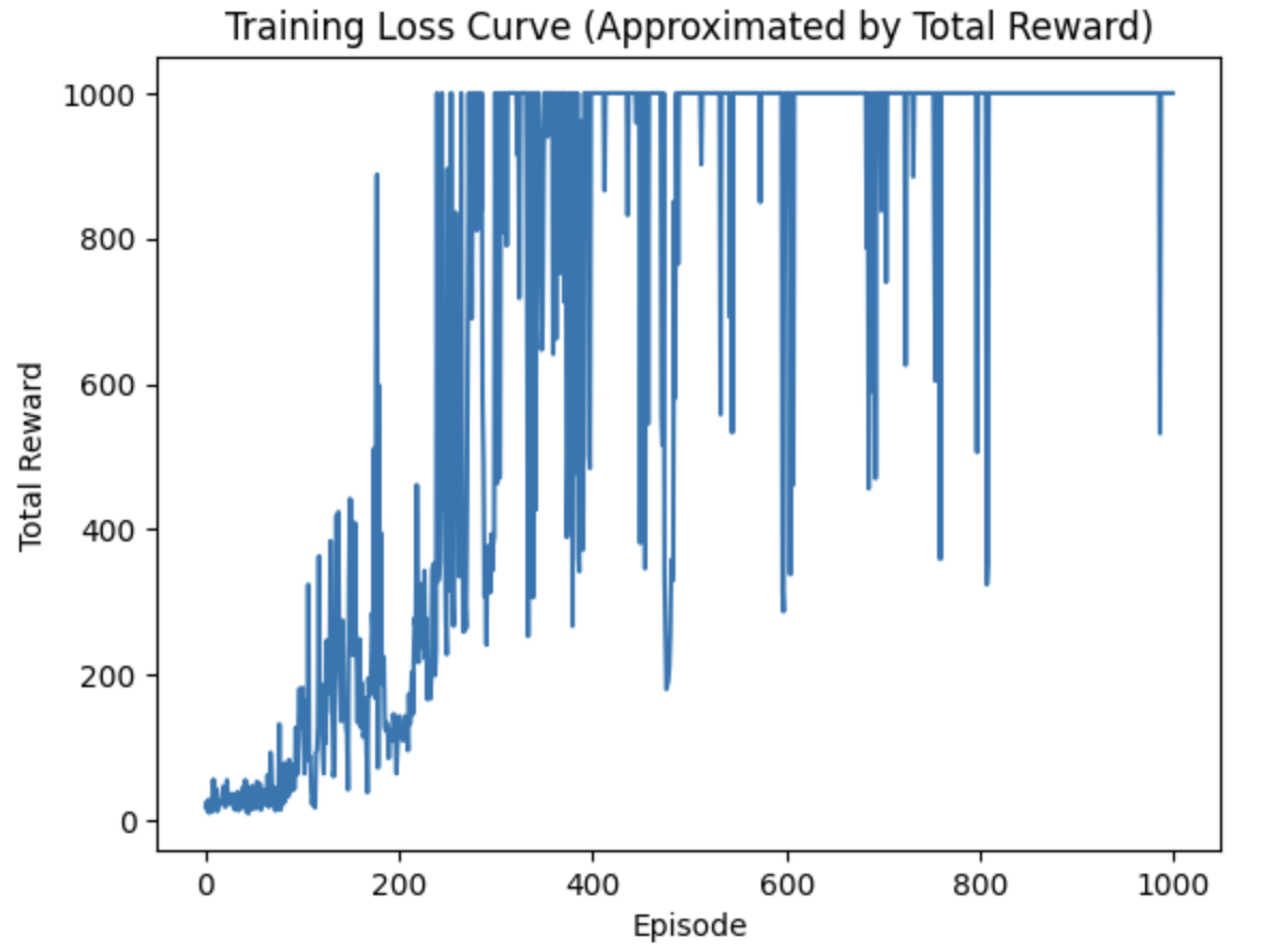
import torch
import torch.nn as nn
import torch.optim as optim
import torch.nn.functional as F
import numpy as np
import gym
from torch.autograd import Variable
from torch.distributions import Categorical
import matplotlib.pyplot as plt
import imageio
from collections import deque

class Actor(nn.Module):
    def __init__(self, num_inputs, num_actions, hidden_size = [128, 64], learning_rate=5e-4):
        super(Actor, self).__init__()

        # 记录动作的数量
        self.num_actions = num_actions
        self.linear1 = nn.Linear(num_inputs, hidden_size[0])
        self.linear2 = nn.Linear(hidden_size[0], hidden_size[1])
        self.linear3 = nn.Linear(hidden_size[1], num_actions)
        # 定义Adam优化器,用于更新网络参数
        self.optimizer = optim.Adam(self.parameters(), lr=learning_rate)

    def forward(self, x):
        x = F.relu(self.linear1(x))
        x = F.relu(self.linear2(x))
        x = self.linear3(x)
        # 使用Softmax函数将输出转换为动作概率分布
        return F.softmax(x, dim=1)


class Critic(nn.Module):
    def __init__(self, num_inputs, output_dim = 1, hidden_size = [128, 64], learning_rate=5e-4):
        super(Critic, self).__init__()

        self.linear1 = nn.Linear(num_inputs, hidden_size[0])
        self.linear2 = nn.Linear(hidden_size[0], hidden_size[1])
        self.linear3 = nn.Linear(hidden_size[1], output_dim)
        # 定义Adam优化器,用于更新网络参数
        self.optimizer = optim.Adam(self.parameters(), lr=learning_rate)

    def forward(self, x):
        x = F.relu(self.linear1(x))
        x = F.relu(self.linear2(x))
        x = self.linear3(x)
        return x

class Agent:
    def __init__(self, n_states, n_actions):

        self.gamma = 0.99
        self.actor = Actor(n_states, n_actions)
        self.critic = Critic(n_states)
        self.memory = deque()
        self.k_epochs = 4
        self.eps_clip = 0.2
        self.entropy_coef = 0.01

    def sample_action(self,state):
        state = torch.tensor(state, dtype=torch.float32).unsqueeze(dim=0)
        probs = self.actor(state)
        dist = Categorical(probs)
        action = dist.sample()
        log_prob = dist.log_prob(action).detach()
        return action.detach().cpu().numpy().item(), log_prob

    @torch.no_grad()
    def predict_action(self,state):
        state = torch.tensor(state, device=self.device, dtype=torch.float32).unsqueeze(dim=0)
        probs = self.actor(state)
        dist = Categorical(probs)
        action = dist.sample()
        return action.detach().cpu().numpy().item()

    def update(self):
        old_states, old_actions, old_log_probs, old_rewards, old_dones = zip(*list(self.memory))
        # convert to tensor
        old_states = torch.tensor(np.array(old_states), dtype=torch.float32)
        old_actions = torch.tensor(np.array(old_actions), dtype=torch.float32)
        old_log_probs = torch.tensor(old_log_probs, dtype=torch.float32)
        # monte carlo estimate of state rewards
        returns = []
        discounted_sum = 0
        for reward, done in zip(reversed(old_rewards), reversed(old_dones)):
            if done:
                discounted_sum = 0
            discounted_sum = reward + (self.gamma * discounted_sum)
            returns.insert(0, discounted_sum)
        # Normalizing the rewards:
        returns = torch.tensor(returns, dtype=torch.float32)
        returns = (returns - returns.mean()) / (returns.std() + 1e-5) # 1e-5 to avoid division by zero
        for _ in range(self.k_epochs):
            # compute advantage
            values = self.critic(old_states) # detach to avoid backprop through the critic
            advantage = returns - values.detach()
            # get action probabilities
            probs = self.actor(old_states)
            dist = Categorical(probs)
            # get new action probabilities
            new_probs = dist.log_prob(old_actions)
            # compute ratio (pi_theta / pi_theta__old):
            ratio = torch.exp(new_probs - old_log_probs) # old_log_probs must be detached
            # compute surrogate loss
            surr1 = ratio * advantage
            surr2 = torch.clamp(ratio, 1 - self.eps_clip, 1 + self.eps_clip) * advantage
            # compute actor loss
            actor_loss = -torch.min(surr1, surr2).mean() + self.entropy_coef * dist.entropy().mean()
            # compute critic loss
            critic_loss = (returns - values).pow(2).mean()
            # take gradient step
            self.actor.optimizer.zero_grad()
            self.critic.optimizer.zero_grad()
            actor_loss.backward()
            critic_loss.backward()
            self.actor.optimizer.step()
            self.critic.optimizer.step()
        self.memory.clear()


# 创建CartPole-v0环境,指定渲染模式为'rgb_array'
env = gym.make('CartPole-v0', render_mode='rgb_array')
# 初始化agent,输入维度为环境观测空间的维度4,输出维度为环境动作空间的维度2,隐藏层大小为128
agent = Agent(env.observation_space.shape[0], env.action_space.n)

# 最大训练回合数
max_episode_num = 1000
# 每个回合的最大时间步数
max_steps = 1000
# 用于记录每个回合的步数
numsteps = []
# 用于记录每个回合的平均步数
avg_numsteps = []
# 用于记录每个回合的总奖励
all_rewards = []

# 开始训练循环
for episode in range(max_episode_num):
    # 重置环境,获取初始状态
    state, _ = env.reset()
    # 用于存储每个时间步的奖励
    rewards = []

    # 在每个回合内进行时间步循环
    steps = 1
    while (True):
        # 渲染环境,显示当前状态`
        env.render()
        # 根据当前状态获取动作和动作的对数概率
        action, log_prob = agent.sample_action(state)
        # 执行动作,获取新的状态、奖励、终止标志等信息
        new_state, reward, done, _, _ = env.step(action)
        agent.memory.append((state, action, log_prob, reward, done))
        # 将奖励添加到列表中
        rewards.append(reward)
        # 如果环境达到终止条件
        if done or steps >= max_steps:
            # 调用更新策略的方法,更新网络参数
            agent.update()
            break
        # 更新当前状态为新的状态
        state = new_state
        steps += 1

    # 计算当前回合的总奖励
    total_reward = sum(rewards)
    all_rewards.append(total_reward)
    if episode % 100 == 0:
        print(f"Episode {episode}: Total Reward = {total_reward}")

# 绘制训练损失曲线(使用总奖励曲线近似表示)
plt.plot(all_rewards)
plt.xlabel('Episode')
plt.ylabel('Total Reward')
plt.title('Training Loss Curve (Approximated by Total Reward)')
plt.savefig('training_loss_curve.png')
plt.show()

# 最后运行一次游戏并保存效果图
frames = []
state, _ = env.reset()
test_reward = 0
for steps in range(1000):
    frame = env.render()  # 去掉mode参数
    frames.append(frame)
    action, _ = agent.sample_action(state)
    new_state, reward, done, _, _ = env.step(action)
    test_reward += reward
    if done:
        break
    state = new_state
print("test_reward: ", test_reward)
env.close()

imageio.mimsave('ppo.gif', frames, fps=30)
reward训练曲线:
最终效果:

 浙公网安备 33010602011771号