Python----朴素贝叶斯

1、朴素贝叶斯

　　朴素贝叶斯是使用概率论来分类的算法。其中朴素：各特征条件独立；贝叶斯：根据贝叶斯定理。

　根据贝叶斯定理，对一个分类问题，给定样本特征B，样本属于类别A的概率是：

2、算法特点

　　优点: 在数据较少的情况下仍然有效，可以处理多类别问题。

　　 缺点: 对于输入数据的准备方式较为敏感。

　　 适用数据类型: 标称型数据。

3、实例

　　

　　

# Importing the libraries
import numpy as np
import matplotlib.pyplot as plt
import pandas as pd

# Importing the dataset
dataset = pd.read_csv('Social_Network_Ads.csv')
X = dataset.iloc[:, [2,3]].values
y = dataset.iloc[:, 4].values

# Splitting the dataset into the Training set and Test set
from sklearn.model_selection import train_test_split
X_train, X_test, y_train, y_test = train_test_split(X, y, test_size = 0.25, random_state = 0)

# Feature Scaling
from sklearn.preprocessing import StandardScaler
sc_X = StandardScaler()
X_train = sc_X.fit_transform(X_train)
X_test = sc_X.transform(X_test)

# Fitting Logistic Regression to the Training set
#从模型的标准库中导入需要的类
from sklearn.naive_bayes import GaussianNB
#创建分类器
classifier = GaussianNB()
#运用训练集拟合分类器
classifier.fit(X_train, y_train)

# Predicting the Test set results
#运用拟合好的分类器预测测试集的结果情况
#创建变量（包含预测出的结果）
y_pred = classifier.predict(X_test)

# Making the Confusion Matrix
#通过测试的结果评估分类器的性能
#用混淆矩阵，评估性能
#65,24对应着正确的预测个数；8,3对应错误预测个数；拟合好的分类器正确率：（65+24）/100
from sklearn.metrics import confusion_matrix
cm = confusion_matrix(y_test, y_pred)

# Visualising the Training set results
#在图像看分类结果
from matplotlib.colors import ListedColormap
#创建变量
X_set, y_set = X_train, y_train
#x1,x2对应图中的像素；最小值-1，最大值+1，-1和+1是为了让图的边缘留白，像素之间的距离0.01；第一行年龄，第二行年收入
X1, X2 = np.meshgrid(np.arange(start = X_set[:, 0].min() - 1, stop = X_set[:, 0].max() + 1, step = 0.01),
                     np.arange(start = X_set[:, 1].min() - 1, stop = X_set[:, 1].max() + 1, step = 0.01))
#将不同像素点涂色，用拟合好的分类器预测每个点所属的分类并且根据分类值涂色
plt.contourf(X1, X2, classifier.predict(np.array([X1.ravel(), X2.ravel()]).T).reshape(X1.shape),
             alpha = 0.75, cmap = ListedColormap(('red', 'green')))
#标注最大值及最小值
plt.xlim(X1.min(), X1.max())
plt.ylim(X2.min(), X2.max())
#为了滑出实际观测的点（黄、蓝）
for i, j in enumerate(np.unique(y_set)):
    plt.scatter(X_set[y_set == j, 0], X_set[y_set == j, 1],
                c = ListedColormap(('orange', 'blue'))(i), label = j)
plt.title('Naive Bayes (Training set)')
plt.xlabel('Age')
plt.ylabel('Estimated Salary')
#显示不同的点对应的值
plt.legend()
#生成图像
plt.show()

# Visualising the Test set results
from matplotlib.colors import ListedColormap
X_set, y_set = X_test, y_test
X1, X2 = np.meshgrid(np.arange(start = X_set[:, 0].min() - 1, stop = X_set[:, 0].max() + 1, step = 0.01),
                     np.arange(start = X_set[:, 1].min() - 1, stop = X_set[:, 1].max() + 1, step = 0.01))
plt.contourf(X1, X2, classifier.predict(np.array([X1.ravel(), X2.ravel()]).T).reshape(X1.shape),
             alpha = 0.75, cmap = ListedColormap(('red', 'green')))
plt.xlim(X1.min(), X1.max())
plt.ylim(X2.min(), X2.max())
for i, j in enumerate(np.unique(y_set)):
    plt.scatter(X_set[y_set == j, 0], X_set[y_set == j, 1],
                c = ListedColormap(('orange', 'blue'))(i), label = j)
plt.title('Naive Bayes (Test set)')
plt.xlabel('Age')
plt.ylabel('Estimated Salary')
plt.legend()
plt.show()

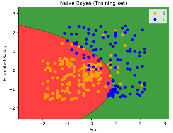
训练集图像显示结果：　　

　　　　　

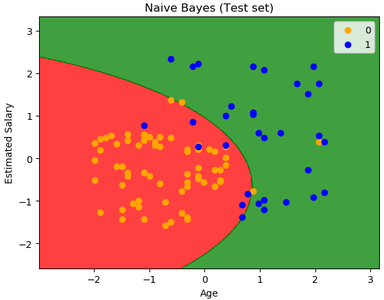
测试集图像显示结果：