
TensorFlow使用记录 (六): 优化器
0. tf.train.Optimizer
tensorflow 里提供了丰富的优化器,这些优化器都继承与 Optimizer 这个类。class Optimizer 有一些方法,这里简单介绍下:
0.1. minimize

minimize(
    loss,
    global_step=None,
    var_list=None,
    gate_gradients=GATE_OP,
    aggregation_method=None,
    colocate_gradients_with_ops=False,
    name=None,
    grad_loss=None
)
- loss: A Tensor containing the value to minimize.
- global_step: Optional Variable to increment by one after the variables have been updated.
- var_list: Optional list or tuple of Variable objects to update to minimize loss. Defaults to the list of variables collected in the graph under the key GraphKeys.TRAINABLE_VARIABLES.
- gate_gradients: How to gate the computation of gradients. Can be GATE_NONE, GATE_OP, orGATE_GRAPH.
- aggregation_method: Specifies the method used to combine gradient terms. Valid values are defined in the class AggregationMethod.
- colocate_gradients_with_ops: If True, try colocating gradients with the corresponding op.
- name: Optional name for the returned operation.
- grad_loss: Optional. A Tensor holding the gradient computed for loss.
compute_gradients(
    loss,
    var_list=None,
    gate_gradients=GATE_OP,
    aggregation_method=None,
    colocate_gradients_with_ops=False,
    grad_loss=None
)
这是优化 minimize() 的第一步,计算梯度,返回 (gradient, variable) 列表。
0.3. apply_gradients
apply_gradients(
    grads_and_vars,
    global_step=None,
    name=None
)
这是优化 minimize() 的第二步,返回一个执行梯度更新的 ops。
TensorFlow使用记录 (八): 梯度修剪 就用到了这两个函数。
1. tf.train.GradientDescentOptimizer
__init__(
    learning_rate,
    use_locking=False,
    name='GradientDescent'
)
标准的梯度下降法优化器。
Recall that Gradient Descent simply updates the weights
by directly subtracting the gradient of the cost function with regards to the weights ( ) multiplied by the learning rate . It does not care about what the earlier gradients were. If the local gradient is tiny, it goes very slowly.
2. tf.train.MomentumOptimizer
__init__(
    learning_rate,
    momentum,
    use_locking=False,
    name='Momentum',
    use_nesterov=False
)
Momentum optimization cares a great deal about what previous gradients were: at each iteration, it adds the local gradient to the momentum vector m (multiplied by the learning rate
), and it updates the weights by simply subtracting this momentum vector.
调用方式:
optimizer = tf.train.MomentumOptimizer(learning_rate=learning_rate, momentum=0.9)
除了标准的 MomentumOptimizer 外,还有一个变体 Nesterov Accelerated Gradient:
The idea of Nesterov Momentum optimization, or Nesterov Accelerated Gradient (NAG), is to measure the gradient of the cost function not at the local position but slightly ahead in the direction of the momentum.
调用方式:
optimizer = tf.train.MomentumOptimizer(learning_rate=learning_rate, momentum=0.9, use_nesterov=True)
3. tf.train.AdagradOptimizer
__init__(
    learning_rate,
    initial_accumulator_value=0.1,
    use_locking=False,
    name='Adagrad'
)
The first step accumulates the square of the gradients into the vector
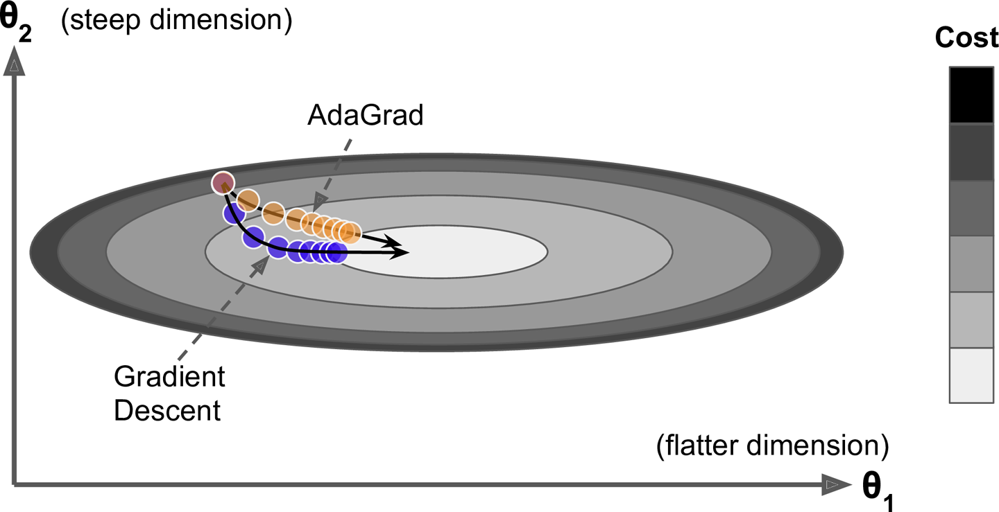
(the symbol represents the element-wise multiplication). This vectorized form is equivalent to computing for each element of the vector ; in other words, each accumulates the squares of the partial derivative of the cost function with regards to parameter . If the cost function is steep along the ith dimension, then will get larger and larger at each iteration. The second step is almost identical to Gradient Descent, but with one big difference: the gradient vector is scaled down by a factor of
(the symbol represents the element-wise division, and is a smoothing term to avoid division by zero, typically set to ). This vectorized form is equivalent to computing for all parameters (simultaneously). In short, this algorithm decays the learning rate, but it does so faster for steep dimensions than for dimensions with gentler slopes. This is called an adaptive learning rate. It helps point the resulting updates more directly toward the global optimum. One additional benefit is that it requires much less tuning of the learning rate hyperparameter
.
调用方式:
optimizer = tf.train.AdagradOptimizer(learning_rate=learning_rate)
不推荐使用:
AdaGrad often performs well for simple quadratic problems, but unfortunately it often stops too early when training neural networks. The learning rate gets scaled down so much that the algorithm ends up stopping entirely before reaching the global optimum. So even though TensorFlow has an AdagradOptimizer, you should not use it to train deep neural networks (it may be efficient for simpler tasks such as Linear Regression, though).
4. tf.train.RMSPropOptimizer
__init__(
    learning_rate,
    decay=0.9,
    momentum=0.0,
    epsilon=1e-10,
    use_locking=False,
    centered=False,
    name='RMSProp'
)
Although AdaGrad slows down a bit too fast and ends up never converging to the global optimum, the RMSProp algorithm14 fixes this by accumulating only the gradients from the most recent iterations (as opposed to all the gradients since the beginning of training). It does so by using exponential decay in the first step.
The decay rate
is typically set to 0.9. Yes, it is once again a new hyperparameter, but this default value often works well, so you may not need to tune it at all.
调用方式:
optimizer = tf.train.RMSPropOptimizer(learning_rate=learning_rate,
                                      momentum=0.9, decay=0.9, epsilon=1e-10)
Except on very simple problems, this optimizer almost always performs much better than AdaGrad. It also generally performs better than Momentum optimization and Nesterov Accelerated Gradients. In fact, it was the preferred optimization algorithm of many researchers until Adam optimization came around.
5. tf.train.AdamOptimizer
__init__(
    learning_rate=0.001,
    beta1=0.9,
    beta2=0.999,
    epsilon=1e-08,
    use_locking=False,
    name='Adam'
)
Adam, which stands for adaptive moment estimation, combines the ideas of Momentum optimization and RMSProp: just like Momentum optimization it keeps track of an exponentially decaying average of past gradients, and just like RMSProp it keeps track of an exponentially decaying average of past squared gradients
is time step. The momentum decay hyperparameter is typically initialized to 0.9, while the scaling decay hyperparameter is often initialized to 0.999. As earlier, the smoothing term is usually initialized to a tiny number such as
调用方式:
optimizer = tf.train.AdamOptimizer(learning_rate=learning_rate)
6. tf.train.FtrlOptimizer
__init__(
    learning_rate,
    learning_rate_power=-0.5,
    initial_accumulator_value=0.1,
    l1_regularization_strength=0.0,
    l2_regularization_strength=0.0,
    use_locking=False,
    name='Ftrl',
    accum_name=None,
    linear_name=None,
    l2_shrinkage_regularization_strength=0.0
)
See this paper. This version has support for both online L2 (the L2 penalty given in the paper above) and shrinkage-type L2 (which is the addition of an L2 penalty to the loss function).


【推荐】编程新体验,更懂你的AI,立即体验豆包MarsCode编程助手
【推荐】凌霞软件回馈社区,博客园 & 1Panel & Halo 联合会员上线
【推荐】抖音旗下AI助手豆包,你的智能百科全书,全免费不限次数
【推荐】博客园社区专享云产品让利特惠,阿里云新客6.5折上折
【推荐】轻量又高性能的 SSH 工具 IShell:AI 加持,快人一步
· Java 中堆内存和栈内存上的数据分布和特点
· 开发中对象命名的一点思考
· .NET Core内存结构体系(Windows环境)底层原理浅谈
· C# 深度学习:对抗生成网络(GAN)训练头像生成模型
· .NET 适配 HarmonyOS 进展
· 本地部署 DeepSeek:小白也能轻松搞定!
· 如何给本地部署的DeepSeek投喂数据,让他更懂你
· 从 Windows Forms 到微服务的经验教训
· 李飞飞的50美金比肩DeepSeek把CEO忽悠瘸了,倒霉的却是程序员
· 超详细,DeepSeek 接入PyCharm实现AI编程!(支持本地部署DeepSeek及官方Dee