


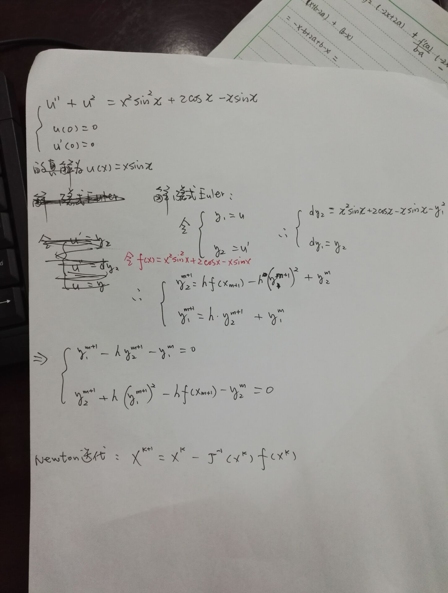
Matlab:高阶常微分三种边界条件的特殊解法(隐式Euler)
函数文件1:
1 function b=F(f,x0,u,h)
2       b(1,1)=x0(1)-h*x0(2)-u(1);
3       b(2,1)=x0(2)+h*x0(1)^2-u(2)-h*f;
函数文件2:
1 function g=Jacobian(x0,u,h)
2   g(1,1)=1;
3   g(1,2)=-h;
4   g(2,1)=2*h*x0(1);
5   g(2,2)=1;
函数文件3:
 1 function x=newton_Iterative_method(f,u,h)
 2  % u:上一节点的数值解或者初值
 3  % x0 每次迭代的上一节点的数值
 4  % x1 每次的迭代数值
 5  % tol 允许误差
 6  % f 右端函数
 7 x0=u;
 8 tol=1e-11;
 9 x1=x0-Jacobian(x0,u,h)\F(f,x0,u,h);
10 while (norm(x1-x0,inf)>tol)
11     %数值解的2范数是否在误差范围内
12     x0=x1;
13     x1=x0-Jacobian(x0,u,h)\F(f,x0,u,h);
14 end
15 x=x1;%不动点
脚本文件:
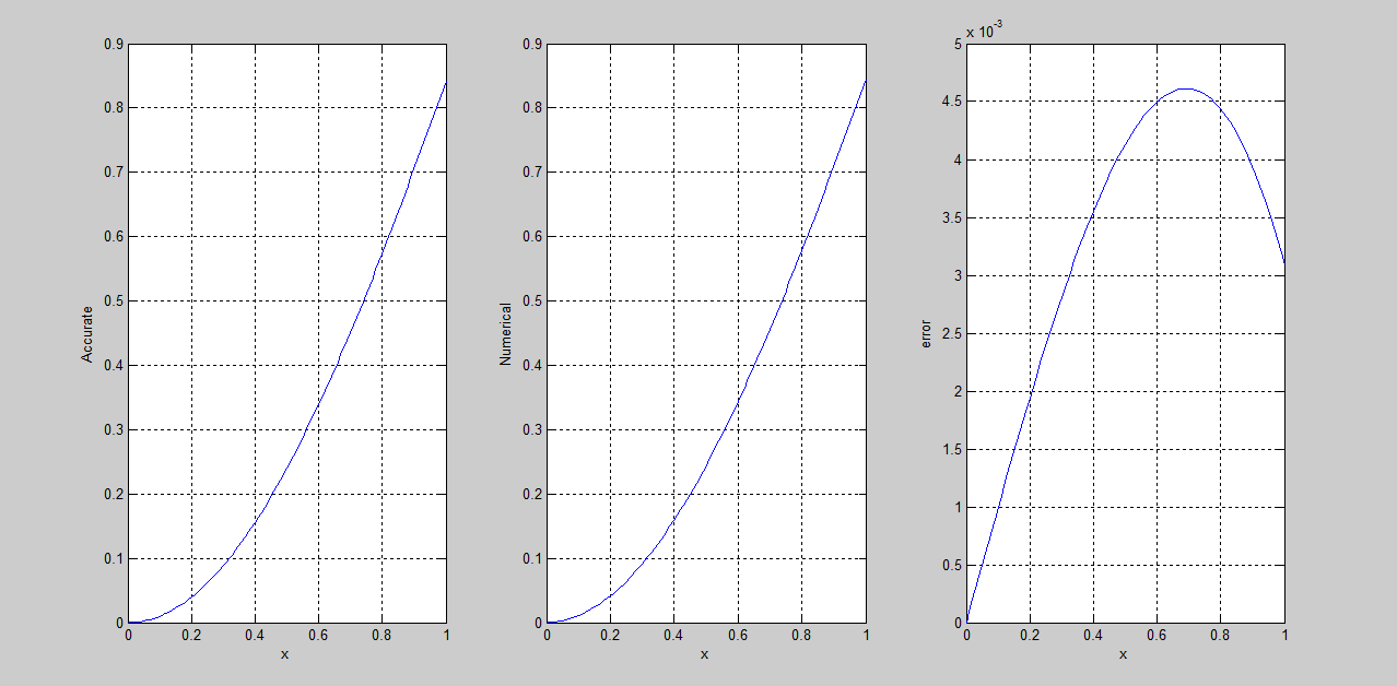
 1 tic;
 2 clear all
 3 clc
 4 N=100;
 5 h=1/N;
 6 x=0:h:1;
 7 y=inline('x.^2.*sin(x).^2+2*cos(x)-x.*sin(x)');
 8 fun1=inline('x.*sin(x)');
 9 Accurate=fun1(x);
10 f=y(x);
11 Numerical=zeros(2,N+1);
12 for i=1:N
13  Numerical(1:2,i+1)=newton_Iterative_method(f(i+1),Numerical(1:2,i),h);
14 end
15 error=Numerical(1,:)-Accurate;
16 subplot(1,3,1)
17 plot(x,Accurate);
18 xlabel('x');
19 ylabel('Accurate');
20 grid on
21 subplot(1,3,2)
22 plot(x,Numerical(1,:));
23 xlabel('x');
24 ylabel('Numerical');
25 grid on
26 subplot(1,3,3)
27 plot(x,error);
28 xlabel('x');
29 ylabel('error');
30 grid on
31 toc;
效果图:
胡冬冬
