概率论与数理统计 Probability Theory and Statistics

概率论与数理统计 Probability Theory and Statistics

Sample space, Event, Event space 样本空间、事件、事件空间

[Def] The set of all possible outcomes is called the sample space. Any subset of the sample space is called an event. Event space is the set of subsets of the sample space.

样本空间：随机变量的所有可能取值的集合是样本空间。
事件：样本空间中的某种结果或多种结果，当试验结果是该种结果或出现在所定义多种结果中的一种，则称试验出现了这个事件。
事件空间：所有可能事件的集合。若样本空间是离散的，则事件空间一般是样本空间的幂集（power set）。

样本空间 vs. 事件：
例1：如试验是掷一次硬币，结果只有两种情况中的一种：正面或反面，则集合 \(\{正面,反面\}\) 即是样本空间，而“{正面}”是一个事件，可表示掷出正面。
例2：试验是投掷2次硬币，样本空间是 \(\{HH,HT,TH,TT\}\) ，其中H表示正面，T表示反面；而“硬币两次面向相同”这样一个事件可表示为集合 \(\{HH,TT\}\) （即两次都是正面或两次都是反面）。

泊松过程（Poisson process）：事件过程以时间序列进行，任意两个不交叠区间的随机量相互独立。

马尔科夫性：将来的状态（当前状态i的下一状态i+1）只与当前状态有关，与以往的状态无关（独立），故P(X=i+1|X=i, X=i-1, ..., X=0)=P(X=i+1|X=i)， 满足马尔科夫性的随机过程叫做马尔科夫链。由现在的状态转移到下一状态的概率称为转移概率。

统计量：将一个样本归结为一个数字，则这个数字就是这个样本的统计量。如均值、方差、中位数。

散点图中的数据展示效果不够理想，则可考虑对数据进行抖动。

概率质量函数 probability mass function, pmf.
The expression \(f(x)=p(X=x)\) for a discrete random variable X is known as the probability mass function.
（离散型随机变量的）概率质量函数值区间一定在[0,1]。

distribution of a discrete random variable: 概率质量函数常被叫做离散型随机变量的分布。

概率密度函数 probability density function, pdf.
A real-valued function \(f: \R^d \mapsto \R, \bm x \mapsto f(\bm x)\) is called a probability density function if

1. \(\forall \bm x \in \R^d, f(\bm x) \geqslant 0\)
2. Its integral exists and

\[p(X\leqslant \bm x)=\int_{-\infty}^{\bm x} f(\bm x)\mathrm{ d }\bm x \\ \int_{\R^d} f(\bm x)\mathrm{d} \bm x = 1 \]

（连续型随机变量的）概率密度函数的值是非负的（概率都是非负的），需要注意其值不一定小于1，函数只要在随机变量状态空间内积分为1即可。

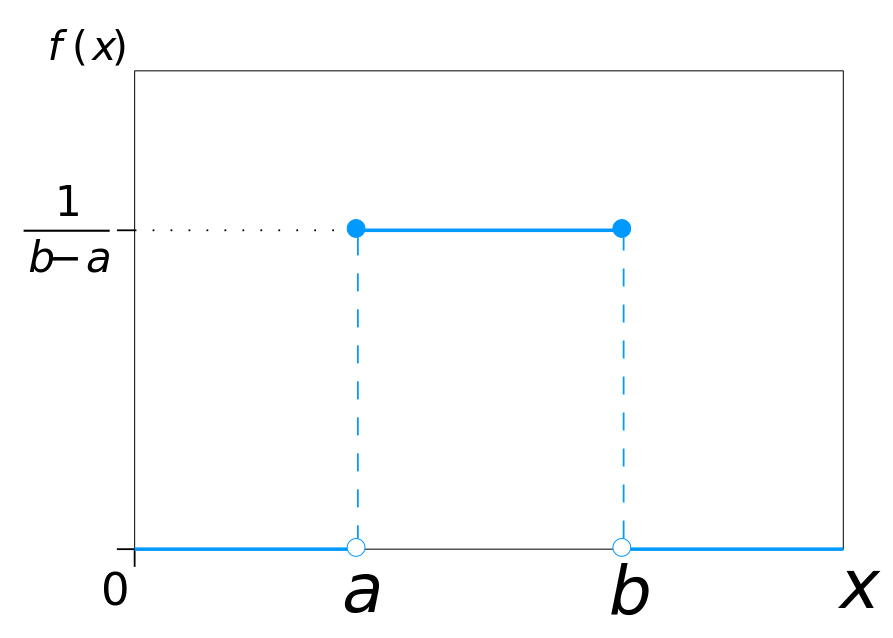
如连续型随机变量X均匀分布在实数区间[1.5,1.9]，则概率密度函数 \(f(x)=2.5\) 并且 \(\int_{1.5}^{1.9} f(x)dx=1\) ，概率密度函数值大于1。

累积分布函数 cumulative distribution function, cdf. The expression \(F(x)=p(X\leqslant x)\) , denoting the probability that a random variable X is less or equal than a particular value \(x\) , is known as the cumulative distribution function. The cdf is non-decreasing (increasing or strictly increasing).

\(p(a\leqslant X \leqslant b)\) denotes the probability that a random variable X is in the interval \([a, b]\) .

连续型随机变量的分布 distribution of a continous random variable：

\[p(a \leqslant X \leqslant b) = \int_a^b f(x) \mathrm d x \]

被称为连续型随机变量的分布。

需要注意的是：和离散型随机变量不同，连续型随机变量在特定值处的概率为0，即 \(p(X=x)=p(x\leqslant X \leqslant x)=\int_x^x f(x)\mathrm d x=0\) ，尽管概率为0但不代表其是不可能事件。

（probability distribution: 累积分布函数有时被叫做连续型随机变量的分布，概率密度函数也有被叫做随机变量的概率分布，得根据上下文来区分它们）

probability integral transform:
Let X be a continuous random variable with a strictly monotonic cumulative distribution function \(F_X(x)\) , then the random variable \(Y\coloneqq F_X(X)\) (i.e. $ y = F_X(x)$ ) has a standard uniform distribution.

Proof:

\[\begin{aligned} F_Y(y) &= P(Y\leqslant y) \\ &= P(F_X(x) \leqslant y) \\ &= P(X\leqslant F_X^{-1}(y)) \\ &= F_X(F_X^{-1}(y)) \\ &= y \end{aligned} \]

其中，因为 \(F_X(\cdot)\) 是严格单调（递增）的，则其反函数 \(F_X^{-1}(\cdot)\) 与其相同也是严格单调（递增）的，从而允许通过 \(P(F_X(x)\leqslant y)\) 推导出 \(P(X\leqslant F_X^{-1}(y))\) .

It is used to derive algorithms for sampling from distributions by transforming transform the result of sampling from a uniform random variable (Bishop, 2006). The algorithm works by first generating a sample from a uniform distribution, then transforming it by the inverse cdf (assuming this is available) to obtain a sample from the desired distribution. The probability integral transform is also used for hypothesis testing whether a sample comes from a particular distribution (Lehmann and Romano, 2005). The idea that the output of a cdf gives a uniform distribution also forms the basis of copulas (Nelsen, 2006).

连续型和离散型随机变量对比：

【离散型】：

\[p(X=x)=\mathrm{pmf}(x) \in [0,1] \\ \sum_{x\in \mathcal X} p(X=x)= \sum_{x\in \mathcal X} \mathrm{pmf}(x) = 1 \\ \text{ 其中 } \mathcal X \text{ 是随机变量的状态空间（目标空间）} \]

【连续型】：

\[p(X=x)=0 \\ \mathrm{pdf}(x)\in [0, \infty) \\ p(X\leqslant x)= \int_{-\infty}^x \mathrm{pdf}(x) \mathrm d x \\ \int_{-\infty}^{+\infty} \mathrm{pdf}(x) \mathrm d x = 1 \\ \mathrm{cdf}(x) \coloneqq p(X\leqslant x)=\int_{-\infty}^x \mathrm{pdf}(x)\mathrm d x \]

随机变量的变换的概率密度（单变元）：

【离散型】
已知离散型随机变量X~P，随机变量Y是X的函数Y:=H(X)，

\[P(Y=y)=P(H(X)=y)=P(X=H^{-1}(y)) \]

【连续型】
借助累积分布函数。累积分布函数、概率密度函数 \(F(\cdot), f(\cdot)\)
，随机变量Y:=H(X)

\[F_Y(y)=P(Y\leqslant y)=P(H(X)\leqslant y) \\ f_Y(y) = \frac{\mathrm d}{\mathrm d y} F_Y(y) \]

如果H(X)严格单调，则

\[f_Y(y)=f_X\left(H^{-1}(y)\right)\left|\frac{\mathrm d}{\mathrm d y} H^{-1}(y) \right| \]

Proof:
假设Y=H(X)是严格递增的，则

\[\begin{aligned} P(H(X)\leqslant y) & = P(X\leqslant H^{-1}(y)) \\ \frac{\mathrm d}{\mathrm d y}H^{-1}(y) & >0 \\ \end{aligned} \\ \Big\Downarrow \\ \begin{aligned} F_Y(y) &= P(Y\leqslant y) \\ &= P(H(X)\leqslant y) \\ &= P(X\leqslant H^{-1}(y)) \texttt{ 其中H递增 } \\ &= \int^{H^{-1}(y)} f_X(x) \mathrm d x \\ &= \int^{H^{-1}(y)} f_X(H^{-1}(y)) \left[\frac{\mathrm d}{\mathrm d y} H^{-1}(y) \right]\mathrm d y \text{ (为抵消下式导数与积分，将微分dx换为dy)} \end{aligned} \\ \Big\Downarrow \\ \begin{aligned} f_Y(y) &= \frac{\mathrm d}{\mathrm d y} F_Y(y) \\ &= \frac{\mathrm d}{\mathrm d y} \int^{H^{-1}(y)} f_X(H^{-1}(y)) \left[\frac{\mathrm d}{\mathrm d y} H^{-1}(y) \right]\mathrm d y \\ &= f_X\left(H^{-1}(y)\right) \left[\frac{\mathrm d}{\mathrm d y} H^{-1}(y) \right] \\ &= f_X\left(H^{-1}(y)\right) \left|\frac{\mathrm d}{\mathrm d y} H^{-1}(y) \right| \end{aligned} \]

若H是严格递减的，则

\[P(H(X)\leqslant y)=P(X\geqslant H^{-1}(y)) = 1-P(X\leqslant H^{-1}(y)) \\ \frac{\mathrm d}{\mathrm d y}H^{-1}(y)<0 \\ \implies \\ \begin{aligned} F_Y(y) &= P(Y\leqslant y) \\ &= P(H(X)\leqslant y) \\ &= P(X\geqslant H^{-1}(y)) \\ &= 1-P(X\leqslant H^{-1}(y)) \texttt{ 其中H递减 } \\ &= 1-\int^{H^{-1}(y)} f_X(x) \mathrm d x \\ &= 1-\int^{H^{-1}(y)} f_X(H^{-1}(y)) \left[\frac{\mathrm d}{\mathrm d y} H^{-1}(y) \right]\mathrm d y \text{ (为抵消下式导数与积分，将微分dx换为dy)} \end{aligned} \\ \implies \\ \begin{aligned} f_Y(y) &= \frac{\mathrm d}{\mathrm d y} F_Y(y) \\ &= \frac{\mathrm d}{\mathrm d y} \left[1- \int^{H^{-1}(y)} f_X(H^{-1}(y)) \left[\frac{\mathrm d}{\mathrm d y} H^{-1}(y) \right]\mathrm d y \right] \\ &= -f_X\left(H^{-1}(y)\right) \left[\frac{\mathrm d}{\mathrm d y} H^{-1}(y) \right] \\ &= f_X\left(H^{-1}(y)\right) \left[-\frac{\mathrm d}{\mathrm d y} H^{-1}(y) \right] \\ &= f_X\left(H^{-1}(y)\right) \left|\frac{\mathrm d}{\mathrm d y} H^{-1}(y) \right| \end{aligned} \]

随机变量的变换的概率密度（多变元）：
Let \(f(\bm x)\) be the value of the probability density of the multivariant continuous random variable X. If the vector-valuaed function \(\bm y=H(\bm x)\) is differentiale and invertible for all values in the domain of \(\bm x\) , then for the corresponding value \(\bm y\) , the probability density of \(Y=H(X)\) is given by

\[f_Y(\bm y)=f_X(H^{-1}(\bm y))\cdot \left| \det \left(\frac{\mathrm d}{\mathrm d \bm y} H^{-1}(\bm y) \right)\right | \]

联合分布的和法则及积法则 （sum rule, product rule）：
假设随机变量X、Y，状态表示x,y，联合分布为p(x,y)，则
【sum rule】

\[p(x)= \begin{dcases} \sum_{y \in \mathcal Y} p(x,y) & \text{ if y is discrete } \\ \int_{y\in \mathcal Y} p(x,y) \mathrm d y & \text{ if y is continuous } \end{dcases} \]

其中 \(\mathcal X, \mathcal Y\) 为目标空间。

【product rule】

\[p(x|y)=\frac{p(x,y)}{p(y)} \]

（准确讲，其中p对于离散型随机变量是指概率质量函数，对于连续型随机变量则指概率密度函数）

【chain rule】(general product rule)

\[p(X_1, X_2,\dots, X_n)=p(X_1|X_2,X_3,\dots, X_n)p(X_2,X_3,\dots,X_n) \\ =p(X_1|X_2,\dots,X_n)p(X2|X_3,\dots,X_n)\dots p(X_{n-2}|X_{n-1},X_n)p(X_{n-1}|X_n)p(X_n) \\ P\left(\bigcap_{i=1}^n X_i\right)=\prod_{i=1}^n P\left(X_i|\bigcap_{j=1}^{i-1}\right) \]

Independence

[Def] Random variables \(X_1,X_2,\dots,X_n\) are said independent if

\[P(X_1=x_1,X_2=x_2,\dots,X_n=x_n)=P(X_1=x1)P(X_2=x_2)\dots P(X_n=x_n), \forall x_1\in \Omega_1,x_2\in\Omega_2,\dots,x_n\in\Omega_n \]

, where \(\Omega_i\) is the sample space of \(X_i\) .

Conditional Independence

[Def] A and B are said conditionally independent if and only if \(P(C)>0\) and

\[P(A|B,C)=P(A|C) \]

, or equivalently

\[P(A,B|C)=P(A|C)P(B|C) \]

.

Conditional Probability

[Def] If \(P(B)>0\) , the conditonal probability of A under condition B is defined as

\[P(A|B)=\frac{P(A\bigcap B)}{P(B)} \]

.

\(P(A|B)\) : read as 'the probability of A given B'.

the marginal likelihood/evidence:

\[p(y) \coloneqq \int p(y,x) \mathrm d x = \int p(y|x)p(x)\mathrm d x = \mathbb E_X [p(y|x)] \]

期望（expectation, expected value）,衡量平均水平：

随机变量的期望：

\[\mathbb E[x] \coloneqq \begin{dcases} \sum_x x p(x) & \text{ if X is discrete} \\ \intop_{\mathcal{X}} x p(x) \mathrm{d}x & \text{ if X is continuous} \end{dcases} \]

随机变量函数 \(f(x)\) 的期望

\[\mathbb E_{X\sim P}[f(x)] \coloneqq \begin{dcases}\sum_{x\in \mathcal X} f(x)p(x) & \text{ if X is descrete} \\ \int_{\mathcal{X}} f(x)p(x) \mathrm{d}x & \text{ if X is continuous} \end{dcases} \]

其中 \(\mathcal X\) 是随机变量的目标空间（所有可能的输出值集合/域）。

协方差（covariance），衡量两个随机变量++线性相关性++的强度：

\[\mathrm{Cov}_{X,Y}[x,y] \coloneqq \mathbb E[(x-\mathbb E[x])(y-\mathbb E[y])] \]

如果协方差的绝对值很大，意味着变量值变化很大，同时距离各自均值很远。如果协方差为正，说明两变量倾向同时取得较大值；如果协方差为负，说明一个变量取较大值时，另一变量倾向取较小值。如果协方差为0，说明两个变量一定没有++线性++相关性（但不排除有非线性关系）。随机变量独立性比协方差为0的要求更强，协方差为0不具备线性相关性，但可能存在非线性依赖。

方差（variance），分布使得函数值f(x)呈现出的差异：

\[\mathrm{Var}(f(x)) \coloneqq \mathbb E[(f(x)-\mathbb E[f(x)])^2]=\mathrm{Cov}[f(x), f(x)] \]

标准差(standard deviation):

\[\sigma=\sqrt{\mathrm{Var}[X]}=\sqrt{\mathbb{E}[(X-\mathbb{E})^2]} \]

变异系数(coefficient of variation):
标准差除以均值得到的比率，“差均比”。

\[\frac{\sigma}{\mu} \]

variation vs. variance:
'variance'是一个统计量，'variation'（尚且）不是一个统计量（即尚未定义严格的数学语义），但'coefficient of variation'是一个统计量。

多元的统计量 multivariate:

期望(多元) Expectation(multivariate):
若多变元随机变量X的状态用 \(\bm x\in \R^d\) 表示，则期望

\[\mathbb E_X[\bm x]=\begin{bmatrix}\mathbb E[x_1] \\ \mathbb E[x_2] \\ ... \\ \mathbb E[x_d] \end{bmatrix} \in \R^d \]

方差（多元） Variance(multivariate): It means covariance generally.

协方差矩阵（covariance matrix）：
对于随机向量（多变元随机变量） \(\bm x\in \mathbb R^n\) ，其协方差矩阵是一个 \(n\times n\) 的矩阵：

\[\mathrm{Cov}(\bm x)_{i,j}=\mathrm{Cov}(x_i,x_j) \]

协方差矩阵对角元是方差： \(\mathrm{Cov}(x_i,x_i)=\mathrm{Var}(x_i)\) 。

协方差矩阵是对称的、正半定的。（symmetric, positive semidefinite）

协方差(多元) Covariance(multivariate), Cross-Covariance:
若两个多变元随机变量X,Y，其状态分别用 \(\bm x\in \R^m, \bm y\in\R^n\) 表示，则协方差

\[\mathrm{Cov}[\bm X, \bm Y]=\mathbb E[(\bm X - \mathbb E[\bm X])(\bm Y-\mathbb E[\bm Y]^T)]=\mathbb E(\bm X\bm Y^T)-\mathbb E[\bm X]E[\bm Y]^T=\mathrm{Cov}[\bm Y, \bm X]^T \in \R^{m\times n}\\ \mathrm{Cov}[\bm x, \bm y]=\mathbb E[\bm x \bm y^T]-\mathbb E[\bm x]E[\bm y]^T=\mathrm{Cov}[\bm y, \bm x]^T \in \R^{m\times n} \]

correlation:

\[\mathrm{corr}[x,y]=\frac{\mathrm{Cov}[x,y]}{\sqrt{\mathrm{Var}[x]\mathrm{Var}[y]}} \in [-1,1] \]

Two random variables \(\bm X, \bm Y\) are called linearly uncorrelated if their covariance is zero \(\mathrm {Cov}[\bm X, \bm Y]=\bm 0\) , or \(\mathbb E(\bm X\bm Y^T]=\mathbb E(\bm X)\mathbb E[\bm Y]^T\) .

运算性质：
若随机变量 \(\bm x, \bm y\) , 常量 \(\bm b, \bm A\) ,仿射 \(\bm A\bm x+\bm b\) ，则

\[\mathbb E[\bm x+\bm y]=\mathbb E[\bm x]+\mathbb E[\bm y] \\ \mathbb E[\bm x+\bm b]=\mathbb E[\bm x]+\bm b \\ \mathbb E[\bm A\bm x+ \bm b]=\bm A \mathbb E[\bm x]+\bm b \\ \mathrm{Var}[\bm x+\bm y]=\mathrm{Var}[\bm x]+\mathrm{Var}[\bm y]+\mathrm{Cov}[\bm x, \bm y]+\mathrm{Cov}[\bm y, \bm x] \\ \mathrm{Var}[\bm x+\bm b]=\mathrm{Var}[\bm x] \\ \mathrm{Var}[\bm A\bm x+\bm b]=\mathrm{Var}[\bm A\bm x]=\bm A\mathrm{Var}[\bm x]\bm A^T \]

经验均值 empirical mean (arithmetic mean)：

\[\bar{\bm x} \coloneqq \frac1N \sum_{n=1}^N \bm x_n \]

where \(\bm x_n \in \R^d\) is the n-th sample in the dataset.

weighted harmonic mean:

\[\bar {x} = \frac{1}{\frac1{\sum_i^n w_i}\sum_i^n \frac{w_i}{x_i}}=\frac{\sum_i^n w_i}{\sum_i^n \frac{w_i}{x_i}} = \frac{w_1 + w_2+\dots + w_n}{\frac{w_1}{x_1}+\frac{w_2}{x_2}+\dots +\frac{w_n}{x_n}} \]

经验方差 empirical variance:

\[\bar {\bm \Sigma} \coloneqq \frac1N \sum_{n=1}^N (\bm x_n - \bar{\bm x})(\bm x_n - \bar{\bm x})^T = \frac1N (\bm X - \bar{\bm x})^T (\bm X - \bar{\bm x}) \]

where \(\bm x_n \in \R^d\) is the n-th sample in the dataset, \(N\) is the number of samples, \(d\) is the dimension of each sample, \(\bm X\in \R^{d\times N}\) is the data matrix, \(\bm X -\bar\bm x\) denotes a matrix whose data vecotr is the difference between the data vector at the corresponding position from \(\bm X\) and \(\bar\bm x\) .

As a special case for centered data matrix( whose mean is zero), empirical variance is

\[\bar{\bm \Sigma}=\frac1N \bm X\bm X^T \]

.

条件概率：

\[p(A|B)\coloneqq\frac{p(A,B)}{p(B)} \]

该定义蕴含着：若一个事件组 \(\{A_1,A_2,...,A_n\}\) 是完备的，则 \(\sum_i^n p(A_i|B)=1\) 。

联合概率 joint probability 在多个随机变量的问题中，若干个随机变量各自的取值情况同时被满足时的概率称为这些随机变量的联合概率。如同时满足两个随机变量X,Y分别取得值X=a,Y=b时的概率称为X=a,Y=b的联合概率，记为p(X=a,Y=b)或更简单的p(a,b)。

若事件A,B是独立的，则 \(p(A,B)=p(A)p(B)\) ， \(p(A|B)=p(A)\) 。

边缘概率(marginal probability)：对应于联合概率，在多变元随机变量问题中，其中一部分变元无关于其他变元的概率。

联合概率的边缘化(marginalisation)：sum rule.

\[p(\bm x)=\int p(\bm x,\bm y)\mathrm d \bm y = \int p(\bm x|\bm y)p(\bm y)\mathrm d \bm y =\mathbb E_{Y} p(X|Y) \\ p(\bm x|\bm \theta)=\int p(\bm x, \bm z|\bm \theta) \mathrm d\bm z=\int p(\bm x|\bm \theta, \bm z) p(\bm z) \mathrm d\bm z \]

联合概率与条件概率：

\[p(A,B)=p(A)p(B|A)=p(B)p(A|B) \]

全概率公式：
若事件组 \({A_1, A_2,...,A_n}\) ，其中两两事件之间是独立的且事件组是完备的，即 $ \forall j\neq k A_j\cap A_k=\varnothing \wedge \sum_i^n p(A_i)=1$ ，则

\[p(B)=\sum_{i=1}^n p(B|A_i)p(A_i) \]

贝叶斯公式(贝叶斯定理 Bayes' Theorem, Bayes' rule, Bayes' law)：

\[\underbrace{p(A|B)}_{\text{posterior}}=\frac{\overbrace{p(B|A)}^{\text{likelihood}}\overbrace{p(A)}^{\text{prior}}}{\underbrace{p(B)}_{\text{evidence}}} \]

or

\[P(H|E,c)=\frac{P(E|H,c)P(H)}{P(E|c)} \]

H: hypothesis
E: evidence
c: context

亦即

\[p(B_i|A)=\frac{p(A|B_i)p(B_i)}{\sum_j^n p(B_j)p(A|B_j)} \]

主要含义是：已知事件A在一个完备事件组B（ \(\{B_1,B_2,...,B_n\}\) ）中各个事件发生下发生的条件概率（即 \(p(A|B_j)\) ），以及事件组中某个事件（ \(B_i\) ）的概率，可据此反过来算出那个事件在A发生下发生的条件概率 \(p(B_i|A)\) 。

According to Bayes’ theorem , the posterior is proportional to the product of the prior and the likelihood.

\[\underbrace{p(A|B)}_{\text{posterior}} \propto \overbrace{p(B|A)}^{\text{likelihood}}\overbrace{p(A)}^{\text{prior}} \]

For a dataset \(\mathcal X\) , a parameters prior \(p(\bm \theta)\) , and a likelihood function \(p(\mathcal X|\bm \theta)\) , the posterior

\[p(\bm \theta|\mathcal X) = \frac{p(\mathcal X|\bm \theta) p(\bm\theta)}{p(\mathcal X)} \\ p(\mathcal X)=\int p(\mathcal X|\bm\theta)p(\bm\theta)\mathrm d \bm\theta \\ p(\bm x)=\int p(\bm x|\bm \theta)p(\bm\theta)\mathrm d\bm\theta = \mathbb E_{\bm \theta}[p(\bm x|\bm\theta)] \]

共轭先验分布 Conjugate Prior Distribution： A prior is conjugate for the likelihood function if the posterior is of the same form/type as the prior.

Table of exmaples of conjugate priors for common likelihood functions:

Likelihood	Conjugate prior	Posterior
Bernoulli	Beta	Beta
Binomial	Beta	Beta
Normal(Gaussian)	Normal / inverse Gamma	Normal / inverse Gamma
Normal	Normal / inverse Wishart	Normal / inverse Wishart
Multinomial	Dirichlet	Dirichlet

logistic sigmoid函数：
logistic sigmoid函数的值域在(0,1)之间。

\[\sigma(x)=\frac1{1+e^{-x}}=\frac1{1+\exp(-x)}=\frac{\exp(x)}{1+\exp(x)} \in (0,1) \frac{d}{dx}\sigma(x)=\sigma(x)(1-\sigma(x))=\sigma(x)\sigma(-x) 1-\sigma(x)=\sigma(-x) \]

softplus函数：

\[\zeta(x)=\log(1+\exp(x)) \]

\[\log\sigma(x)=-\zeta(-x) \frac d{dx}\zeta(x)=\sigma(x) \forall x\in(0,1),\; \sigma^{-1}(x)=\log\left(\frac1{1-x}\right) \zeta(x)-\sigma(x)=x \]

函数 \(\sigma^{-1}(x)\) 在统计学中被称为分对数（logit, log 'it'）。

中心极限定理：
独立同分布的n个随机向量的均值（也是随机变量）在n趋向无穷时，均值随机变量的分布趋近正态分布。

Eigenvalues of a Right Stochastic Matrix

A right stochastic matrix is a square matrix \(\bm A\in \R^{n\times n}\) with all entries non-negative and each row vector summing up to 1.

\[\bm A \ge 0 \wedge \forall i\in [1,n]:\sum_j A_{ij}=1 \]

Properties of a right stochastic matrix:

• A stochastic matrix has an eigenvalue 1.
• The absolute value of any eigenvalue of a stochastic matrix is less than or equal to 1.
• \(\lim_{n\to \infty} A^n\) for a stochastic matrix \(A\) will converge.

++各向同性++的分布（如高斯分布），是指独立同分布，均值、方差（离散度）相同。

Law of Large Numbers 大数定律

Weak Law of Large Numbers

样本量越多，则样本均值越接近真实均值。

[Def] sample mean: For i.i.d. random variables \(X_1, X_2,\dots, X_n\) , the sample mean is defined as

\[\bar X_n := {1\over n}\sum_i^n X_i \]

, which is also a random variable.

Note that, we have

\[\begin{aligned} \mathbb E[\bar X_n] &= \mathbb E\left[{1\over n} \sum_i^n X_i\right] \\ &={1\over n} \sum_i^n \mathbb E[X_i] & \text{ by linearity of expectation} \\ &= {n \mu \over n} \\ &= \mu \end{aligned} \begin{aligned} {\rm{Var}}(\bar X_n) &= {\rm{Var}}\left[{1\over n} \sum_i^n X_i\right] \\ &= {1\over n^2} \sum_i^n {\rm{Var}}[X_i] & \text{ Xi's are independent} \\ &= {\sigma^2\over n} \end{aligned} \]

, where \(\mu\) denotes the expectation of \(X_i\) 's, or \(\mu:= \mathbb E[X_i]\) , and \(\sigma^2 := {\rm{Var}}[X_i]\) .

\[\forall \epsilon >0: \lim_{n \to \infty } \mathrm{P}\left(\left|\frac1n \sum_i^n X_i - \mathbb E[X]\right|< \epsilon\right) = 1 \]

or

\[\bar X_n \overset{P}{\to} \mathbb E[X] \]

The sample average converges in probability towards the expectation.

Strong Law of Large Numbers

\[P(\lim_{n\to \infty} \bar X_n = \mu) = 1 \]

切比雪夫不等式 Chebyshev's inequality：
如果随机变量的期望和方程存在且有限， \(\mathbb E(X)=\mu, D(X)=\sigma^2\) ，则

\[\forall \varepsilon >0, P(|X-\mu|\ge\varepsilon)\le\frac{\sigma^2}{\varepsilon^2} \]

。

可用切比雪夫比等式证明大数定律。

依概率收敛： 设有随机变量序列 \(X_1,X_2,\dots, X_n\) ，以及随机变量 \(X\) ，当满足下式时称序列依概率收敛于 \(X\) ：

\[\forall \epsilon>0: \lim_{n\to \infty} P(|X-X_n|<\epsilon) = 1 \]

。

Moran's Index

Moran's Index is a measure of spatial autocorrelation.

Naive Bayes Classifier

There is a strong assumption: the features of a sample are independent, and values of features are descrete:

\[p(X_1,X_2,\dots, X_n) = \prod_i^n p(X_i) \]

, where \(X_i\) is the random variable of the \(i\) -th feature of a sample, and \(n\) is the number of features of samples.

The predicted class for an input sample \(\bm x\) is given by

\[\begin{aligned} \hat y &= \argmax_{c_k} p(Y=c_k|X=\bm x) \\ &=\argmax_{c_k} \frac{p(X=\bm x|Y=c_k)p(Y=c_k)}{p(X=\bm x)}\\ &=\argmax_{c_k} p(X=\bm x|Y=c_k)p(Y=c_k) \\ &=\argmax_{c_k} p(Y=c_k) \prod_i^n p(X_i=x_i|Y=c_k) \end{aligned} \]

.

The conditional probabilities \(p(X_i|Y)\) and the class probability \(P(Y)\) can be learned from datasets, or simply estimated by frequency

\[p(Y=c_k) = \frac{\mathrm{count}(Y=c_k)}{\sum_{k'}^K \mathrm{count}(Y=c_{k'})} p(X_i=x_i|Y=c_k) = \frac{\mathrm{count}(X_i=x_i,Y=c_k)}{\sum_{x_i'\in\Omega_i} \mathrm{count}(X_i=x'_i, Y=c_k)} \]

, where \(\Omega_i\) denotes the sample space of the random variable \(X_i\) (i.e. the all possible descrete values of the i-th feature).

To avoid zero probabilities due to unseen data, we use smoothing tricks:

\[p(X_i=x_i|Y=c_k) = \frac{\mathrm{count}(X_i=x_i,Y=c_k) + \lambda}{\sum_{x_i'\in\Omega_i} \mathrm{count}(X_i=x'_i, Y=c_k) + |\Omega_i|\lambda} \]

. If \(\lambda=1\) , it is Laplace smoothing (add-1 smoothing).

MaxEnt Model 最大熵模型

\[\begin{aligned} \max_P && & H(P) = -\sum_{x\in \mathcal X} P(x) \log P(X) \\ \text{s.t.} && & \mathbb E_{X\sim P}(f_i(X)) = \mathbb E_{X\sim \tilde P}(f_i(X)) \end{aligned} \]

, for unsupervised datasets, where \(\tilde P\) is emperical distribution, \(f_i\) 's are feature functions.

\[\begin{aligned} \max_P && & H(P) = -\sum_{x\in \mathcal X, y\in \mathcal Y} \tilde P(x) P(y|x) \log P(y|x ) \\ \text{s.t.} && & \mathbb E_{\sim P} [f_i(x,y)] =\mathbb E_{\sim\tilde P} [f_i(x,y)], \forall i \\ && & \sum_y P(y|x) = 1 \end{aligned} \]

, for supervised datasets, where \(\tilde P\) is emperical distribution, \(f_i\) 's are feature functions.

In general, form of maximum entropy model:

\[P(y|x; w) = \frac1{Z_w(x)}\exp\left(\sum_i w_i f_i(x,y)\right) Z_w(x)=\sum_y \exp \left(\sum_i w_i f_i(x,y)\right) \]

.

Distributions

Uniform Distribution

均匀分布 Uniform Distribution:

Normal Distribution, Gaussian Distribution

正态分布 (Normal Distribution, 高斯分布 Gaussian Distribution)：

\[\mathcal N(x;\mu,\sigma^2)=\sqrt{\frac1{2\pi\sigma^2}}\exp\left(-\frac1{2\sigma^2}(x-\mu)^2\right) \\ \mathcal N(\bm x;\bm\mu,\bm \Sigma^{-1})=\sqrt{\frac{\det(\bm\Sigma)}{(2\pi)^n}}\exp\left(-\frac12(\bm x-\bm\mu)^T\bm\Sigma(\bm x-\bm\mu)\right) \]

where \(\bm x\in\R^n\) , \(\bm\Sigma\) is symmetric, postive semidefinite.

Standard Normal Distribution: \(\mathcal N (0,1)\)

standarlizing a general normal distribution:

\[\mathcal x\sim N (\mu,\sigma^2) \implies \frac{x-\mu}{\sigma} \sim \mathcal N(0, 1) \]

If X, Y are independent (so the joint probability is given as \(p(x,y)=p(x)p(y)\) ) and both follow the normal distribution, \(X \sim \mathcal N(\bm x|\bm\mu_x, \bm\Sigma_x), Y\sim \mathcal N(\bm y|\bm\mu_y, \bm\Sigma_y)\) , then the \(X+Y\) , i.e. \(\bm x+\bm y\) also follows the normal distribution \((X+Y) \sim \mathcal N(\bm x+\bm y | \bm\mu_x + \bm\mu_y, \bm\Sigma_x+\bm\Sigma_y)\) .

affine transformation of the multivariate normal distribution:

Let \(X\) be a multivariate random variable of a normal distribution \(\mathcal N(\bm\mu_X, \bm\Sigma_X)\) , then the affine transformation \(Y=\bm WX+\bm b\) is a random variable from a normal distribution with the mean \(\bm\mu_Y=\bm W\bm\mu_X+\bm b\) , and the variance \(\bm\Sigma_Y=\bm W\bm\Sigma_X \bm W^T\) , or

\[X\sim \mathcal N(\bm\mu, \bm\Sigma), Y=\bm WX+\bm b \\ \Downarrow \\ Y\sim \mathcal N(\bm W\bm \mu, \bm W\bm\Sigma\bm W^T) \]

Bernoulli Distribution 伯努利分布

一次试验的结果只能为二者中的一种，非此即彼。

Bionomial Distribution 二项分布

一次试验过程可分为n次重复“子过程”，该子过程是一个伯努利过程，即其结果状态为“是、否”二者中的一种，二项分布概率函数是描述在一次试验中对于重复子过程数量为n的情况，试验结果出现k次“是”（蕴含出现n-k次“否”）的概率。

如，我们可能关心这样的场景：一次试验是扔硬币100次（即n=100），那硬币正面出现的次数为50次的概率是多少？出现20次的概率又是多少？
或者另一个例子：我们设计了一个很奇怪的随机模型，其不论输入是什么都随机地输出0或1，那对于有100个输入的数据集（n=100），那模型输出结果1出现50次的概率是多少？

Log-Normal Distribution

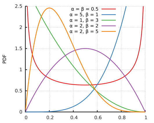
Beta Distribution

The Beta distribution is a distribution over a continuous random variable \(x\in [0,1]\) which is often used to represent the probability for some binary event.

\(X\sim \mathrm{Beta}(\alpha, \beta)\)

点估计、区间估计

估计的偏差：

\[\text{bias}(\hat\bm\theta_m)=\mathbb E(\hat\bm\theta_m)-\bm\theta \]

m为样本量。
如果 \(\text{bias}(\hat\bm\theta)=0\) 则称估计量 \(\hat\bm\theta\) 是++无偏++的。如果 \(\lim_{m\to\infty}\text{bias}(\hat\bm\theta)=0\) 则称估计量是++渐近无偏++的。

伯努利分布的样本均值是分布真实均值的无偏估计。

正态分布中，样本方差 \(\hat\sigma^2_m=\frac1m\sum_{i=1}^m(x^{(i)}-\hat\mu_m)^2\) 是分布的真实方差 \(\sigma^2\) 的有偏估计，偏差为 \(-\sigma^2/m\) 。真实方差的无偏估计为 \(\tilde\bm\theta_m=\frac1{m-1}\sum_{i=1}^m(x^{x(i)}-\hat\mu_m)^2\) ，称为无偏样本方差，其中 \(\hat\mu_m\) 是样本均值。

Gamma Distribution, Γ

Chi-Squared Distribution, χ²

References:

• https://en.wikipedia.org/wiki/Chi-square_distribution

Gumbel Distribution

(generalized extreme value distribution Type-I)

概率图模型 Graphical Models

概率图模型：
朴素贝叶斯分类器；
隐马尔可夫模型；
线性回归；
d-分离（d-separation）；
信念传播；（链、树、多树、结树）；
马尔可夫随机场（无向图）；
影响图（influence diagram）；

贝叶斯网络(Bayesian Network)

有向图概率模型 Directed Graphical Model。

其是一个有向无环图（DAG）。

A Bayesian network satisfies the local Markov property, which means that the probability of a node is conditionally independent only upon its parents and not upon any non-descendants.

conditionally independent: 'A is conditionally independent of B given C' is denoted by

\[A\perp\!\!\!\perp B | C \]

条件性地独立的典型情况：

1. 头尾连接 head-to-tail connection

graph LR
    X-->Y
    Y-->Z

\[ \]

这种情况的意味着，给定Y时，X和Z是独立的，即 \(p(X,Z | Y)=p(X|Y)p(Z|Y)\) 。联合概率 \(p(X,Y,Z)=p(X)p(Y|X)p(Z|Y)\) 。

2. 尾尾连接 tail-tail

graph TD
    X-->Y
    X-->Z

这种情况的意味着，：给定X时（X发生的条件下）Y和Z是独立的，即 \(p(Y,Z|X)=p(Y|X)p(Z|X)\) 。联合概率 \(p(X,Y,Z)=p(X)p(Y,Z|X)=p(X)p(Y|X)p(Z|X)\) 。

3. 头头连接 head-to-head

graph TD
    X-->Z
    Y-->Z

这种情况的意味着，已知Z时X和Y是依赖的。合概率 \(p(X,Y,Z)=p(X,Y)p(Z|X,Y)=p(X)p(Y)p(Z|X,Y)\) 。

联合概率示例：

graph TD
    X1 --> X3
    X2-->X3
    X2-->X4
    X5-->X2

the joint probability:

\[p(x_1,x_2,x_3,x_4,x_5)=p(x_1)p(x_5)p(x_3|x_1,x_2)p(x_2|x_5)p(x_4|x_2) \]

In general, the joint probability distribution \(p(\bm x)=p(x_1,...,x_n)\) for random variables (i.e. nodes) \(x_1,x_2, \dots, x_n\) is given by

\[p(\bm x)=\prod_{i=1}^n p(x_i | \text{parent-nodes-of } x_i) \]

The simplest form of a Bayesian network is a Naive Bayesian classifier.

References:

• https://towardsdatascience.com/introduction-to-bayesian-networks-81031eeed94e?gi=a750932e1af6
• Introduction and Applications: https://scholarship.claremont.edu/cgi/viewcontent.cgi?article=2690&context=cmc_theses

Markov Process

A Markov process in the domain of probability is a stochastic process satifying the Markov proerty, with which the conditional probability depends only upon the most recent one state (the previous state) and deos not depdend on more ealier states.

Markov property

In the domain of probability and statistics, a stochastic process has the The Markov property if the conditional probability of the future state depends only upon the present state. i.e.

\[p(s_t|s_{t-1}s_{t-2}s_{t-2}\cdots) = p(s_t|s_{t-1}) \]

A discrete-time stochastic process with Markov property is known as a Markov chain.

A Markov random field extends the Markov property to two or more variables.

Transition Kernel

(continous Markov model)

A funtion \(k(x, A)\) is a transition kernel for \(x\in S\) (may be discrete or continous) and \(A\in B(S)\) where \(B(S)\) is a σ−field on \(S\) such that:

• \(k(x, \cdot)\) is a probability measure for all \(x\in S\)
• \(k(\cdot, A)\) is measurable for all \(A\in B(S)\) .

Or definition:
The transition kernel for \(x\in S\) and \(A\in B(S)\) where \(B(S)\) is a σ−field on \(S\) is defined as a conditional density function:

\[k(x,A)=P(X\in A|x)=\int_{x'\in A} k(x,x') dx' \]

, where \(X\) is the random variable for the first argument of \(k\) , \(P(\cdot|\cdot)\) is the conditional probability density function, \(k(x, x')\) is a function on \(S\times S\) and is also called a transition kernel.

References:

• https://www.math.kth.se/matstat/gru/sf2955/metropolisB3.pdf

Hidden Markov Model (HMM) 隐马尔可夫模型

离散马尔可夫过程：一个系统，其在任意时刻会处于且只能处于N个状态中的一个。记状态集为 \(S=\{S_1, S_2, ..., S_N\}\) ，系统在时刻t时的状态为 \(q_t\) ，意味着 \(q_t=S_i\in S, 1\leqslant i \leqslant N\) 。这里的时刻的内涵在于其是某种序列上的一点，该方法可对任意序列都有效，如时序、空间轨迹等。

系统在离散的时刻根据以前的状态以既定的概率转到下一个状态：

\[p(q_{t+1}| q_t, q_{t-1}, ...) \]

对于一阶马尔可夫模型，系统在下一个时刻的状态仅依赖于当前时刻的状态，而与更早的状态无关：

\[p(q_{t+1} | q_t, q_{t-1}, ...) = p(q_{t+1} | q_t) \]

转移概率：系统从一个状态转移到另一个状态的概率。可以简化模型，假设状态间的转移概率与系统发展过程无关（即与时间无关），亦即 \(p(q_{t+1}|q_t)\equiv p(q_{t'+1}|q_{t'}), \forall t, t'\) 。转移概率矩阵 \(\bm A_{N\times N}\) ，其中元素 \(A_{ij}\) 表示从状态i转移到状态j的概率，由于一个状态i到所有可能的状态（包括相同的状态i）的转移概率之和应该为1，故 \(A_{ij}\ge 0 \wedge \sum_j A_{ij}=1\)

在一个可观测的马尔可夫模型（observable Markov model）中，状态是可被观测的，在任意时刻t，我们都可知道其对应的状态 \(q_t\) ，并随着过程的发展，系统不断地从一个状态转移到另一个状态。

隐马尔可夫模型：
Hidden Markov Model, HMM。在隐马尔可夫模型中，系统的状态是不可被观测的，但是系统到达一个状态时，可以记录一个观测，这个观测是此时系统状态的一个概率函数。

HMM中假设状态转移概率不依赖于时间t，即在任何时候，从状态 \(q_i\) 转移到状态 \(q_j\) 的概率均相同。

模型可能的状态的集合记S，可能的观测结果种类的集合记V。模型状态序列记Q，观测序列记O。时间t时，模型状态为 \(q_t\) ，观测（结果）为 \(O_t\) 。初始时刻的状态记 \(q_1\) 。

对于一个既定模型，一个同样的观测序列可以由多个不同的状态序列产生而来，但我们一般只关心具有最大概率产生观测序列的那个状态序列。

形式化HMM：

1. 模型状态集S。状态集记为 \(S=\{S_1, S_2, ..., S_N\}\) ，设有N种可能状态。
2. 观测结果种类集V。观测结果种类集合记 \(V=\{v_1, v_2, ..., v_M\}\) ，设有M种可能类别，观测序列的元素即从该集合中取样。
3. 状态转移概率 (transition probability matrix)：

\[\bm A = [a_{ij}]\in\R^{N\times N}, \text{ 其中 } a_{ij}\equiv p(q_{t+1}=S_j | q_t=S_i), \forall t \]

其中的“恒等且对所有t”（ \(...\equiv ... \forall t\) ）即表示转移概率与时间无关，HMM假设转移概率与时间（前序观测结果）无关（从观测序列的隐状态序列角度看即是当前隐状态仅与上一个隐状态有关，与更早的隐状态无关，不由历史可观测结果决定）。
4. 观测概率 (emission probability matrix, observation likelihoods)

\[\bm B=[b_{jm}]\in\R^{N\times M}, \text{ 其中 } b_{jm}\equiv p(O_t=v_m | q_t=S_j), \forall t \]

即模型隐状态为 \(S_j\) 时，观测结果的种类为 \(v_m\) 的概率，在任意时刻均如此，HMM中假设其与时间无关，即假设任意时刻上的观测 \(o_t\) 的结果仅由其隐状态 \(s_t\) 有关，与前序观测结果无关。
5. 观测序列O。 \(O=[o_1, o_2,\cdots, o_T]\) ，一个观测值 \(o_t\) 从集合V中取样，其还隐含一个不可观测的状态 \(q_t\) （即HMM中的hidden variable）。
6. 初始时刻各状态概率：

\[\bm\Pi = [\pi_i]\in\R^N, \text{ 其中 } \pi_i = p(q_1=S_i), 1\le i \le N, \sum_{i}^N \pi_i = 1 \]

\(\lambda=\left(\bm A, \bm B, \bm \Pi\right)\) 被称作HMM的参数集（其中蕴含了N，M）。

HMM关心的3类问题：

1. 估计指定观测序列的概率（Likelihood）。已知模型 \(\lambda\) ，希望估计出指定观测序列 \(O=<O_1, O_2, ..., O_T>\) 的概率，即 \(p(O|\lambda)\) 。
2. 找出状态序列 \(Q\) （Decoding）。已知模型 \(\lambda\) 以及一个观测序列O，希望找出状态序列 \(Q=<O_1,O_2,...,O_T>\) ，可能的解会有若干个，但我们只关心其中具有最大概率产生观测序列O的那个状态序列 \(Q^*\) ，即

\[Q^* = \arg\max_Q p(O| Q,\lambda) \]

3. 找出模型参数 \(\lambda\) （Learning）。已知以观测序列组成的训练集 \(\mathcal X={O^{(k)}}\) （即其中一个样本k是一个观测序列 \(O^{(k)}=<O_1^{(k)},O_2^{(k)},...>\) ），希望学习到具有最大概率产生 \(\mathcal X\) 的模型参数 \(\lambda^*\) ，即

\[\lambda^* = \arg\max_\lambda p(\lambda | \mathcal X) \]

The joint probability of a HMM:
using notation from sequence classification problems, \(\bm x=[x_1,x_2,\dots, x_T]\) for an input sequence (observation sequence) with sequence length \(T\) , and \(\bm y=[y_1,y_2,\dots,y_T]\) for labels (hidden sequence).

\[\begin{aligned} p(\bm y, \bm x)&=p(\bm x|\bm y)p(\bm y) && \text{ (1) }\\ &= p(x_1,x_2,\dots, x_T|\bm y)p(\bm y) \\ &= \prod_{t=1}^T p(x_t|\bm y) p(\bm y) && \text{ (3) } \\ &=\prod_{t=1}^T p(x_t|y_1,y_2,\dots,y_T) p(\bm y) \\ &= \prod_{t=1}^T p(x_t|y_t) p(\bm y) && \text{ (5) } \\ &=\prod_{t=1}^T p(x_t|y_t) p(y_1,y_2,\dots,y_T) \\ &= \left[\prod_{t=1}^T p(x_t|y_t)\right] \left[\prod_{t=1}^T p(y_t|y_1,\dots,y_{t-1})\right ] && \text{ (7) } \\ &=\left[\prod_{t=1}^T p(x_t|y_t)\right] \left[\prod_{t=1}^T p(y_t|y_{t-1})\right ] && \text{ (8) } \\ &=\prod_{t=1}^Tp(x_t|y_t)p(y_t|y_{t-1}) \end{aligned} \]

(1): by Bayes' rule
(3): by HMM assumption: independence between observation
(5): by HMM assumption: an observation is only dependent on the corresponding hidden state
(7): by Bayes' rule
(8): by HMM assumption: a hidden state is only dependent its previous hiddent state

HMM from the Bayesian network prespective:

(where \(n\) is the length of the sequence, equal to \(T\) above)

the joint probability according to Bayesian network:

\[\begin{aligned} p(\bm y, \bm x) &= \prod_{t=1}^T (\text{node}_t | \text{parents-node-t}) \\ &=\prod_{t=1}^T p(x_t|y_t) \prod_{t=1}^T p(y_t|y_{t-1}) \\ &=\prod_{t=1}^T p(x_t|y_t) p(y_t|) \end{aligned} \]

Viterbi - HMM decoding algorithm

Viterbi in HMM:
recursive step

\[ \alpha_{t+1}(s)=\sum_{s'\in S} \alpha_t (s')p(q_{t+1}=s|q_t=s')p(o_{t+1}|q_t=s) \]

, where \(\alpha_t(s)\) denotes the probability of producing the observation sequence up to time \(t\) and the hidden state being \(s\) at time \(t\) .

Baum-Welch - HMM training algorithm

Maximum Entropy Markov Models, MEMM

Viterbi recurve step for MEMM:

\[\alpha_{t+1}(s)=\sum_{s'\in S} \alpha_t(s')p(s|s', o_{t+1}) \]

.

Maximum entropy is a framework for estimating probability distributions from data. It is based on the principle that the best model for the data is the one that is consistent with certain constraints derived from the training data, but otherwise makes the fewest possible assumptions.

HMM vs. MEMM:
HMMs are generative, and MEMMs are discriminative.

Markov Random Fields 马尔科夫随机场

A Markov random field is a set of random variables having the Markov property described by an undirected graph.

A Markov random field is known as a Markov network or undirected graph model. (无向图概率模型)

Differences between Markov networks and Bayesian networks: Bayesian networks are directed and acylic, and Markov networks are undirected and may be cylic.

e.g.:
A multivariate normal distribution forms a Markov random field \(G=(V,E)\) if the pair nodes of a zero entry inside the inverse covariance matrix corresponds to the unreachability between the pair nodes. i.e.:

\[\bm X=[\bm X_v]_{v\in V} \sim \mathcal{N}(\bm \mu, \bm \Sigma) \]

such that

\[[\bm \Sigma^{-1}]_{uv} = 0 \iff <u,v>\not\in E \]

.

Conditional Random Field (CRF)

Linear chain conditional random field

[Lafferty et al., 2001]

CRFs make independence assumptions among \(\bm y\) , but not among \(\bm x\) .

CRFs are probabilistic graphical models which combine the advantage of generative models and discriminative models.

The reason we distinguish graphical models from regular probabilistic models for sequence analying task is that the target search space is too large for regular probilistic models and we want to benifit better inference and search effiency from graphical models.

[Def] Let X,Y be random vectors, \(\bm \lambda=[\lambda_k]\in\R^K\) be a parameter vector, \(\{f_k(y,y', x_t)\}_{k=1}^K\) be a set of real-valued feature functions. Then a linear chain conditional random field is a conditional probability distribution

\[p(\bm y|\bm x)=\frac{1}{Z(\bm x)} \exp \left\{\sum_{k=1}^K \lambda_k f_k(y_t, y_{t-1}, x_t)\right\} \]

, where \(Z(\bm x)\) is an instance-specific normalization factor

\[Z(\bm x)=\sum_{\bm y} \exp \left\{\sum_{k=1}^K\lambda_k f_k(y_t, y_{t-1}, x_t)\right\} \]

(Z(x) sums over all possible state sequences).

objective function for a sample \(\bm x^{(i)}, \bm y^{(i)}\) :

\[l(\bm \lambda; \bm x^{(i)},\bm y^{(i)}) = \log p(\bm x^{(i)}| \bm y^{(i)}) - \frac{1}{2\sigma^2} \|\bm \lambda\|_2^2 \\ =\sum_t^T \sum_k^K \lambda_k f_k (y_t^{(i)}, y_{t-1}^{(i)}, \bm x_t^{(i)}) - \log Z(\bm x^{(i)}) - \frac{1}{2\sigma^2} \|\bm \lambda\|_2^2 \]

objective funtion over the whole dataset:

\[L(\bm \lambda) = \sum_i^N\log p(\bm x^{(i)}| \bm y^{(i)}) - \frac{1}{2\sigma^2} \|\bm \lambda\|_2^2 \\ =\sum_i^N \sum_t^T \sum_k^K \lambda_k f_k (y_t^{(i)}, y_{t-1}^{(i)}, \bm x_t^{(i)}) - \sum_i^N \log Z(\bm x^{(i)}) - \frac{1}{2\sigma^2} \|\bm \lambda\|_2^2 \]

the derivative with respect to the parameter is

\[\frac{\partial L}{\partial \lambda_k}=\sum_i^N \sum_t^T f_k(y_t, y_{t-1}, x_t) - \sum_i^N \sum_t^T \sum_{y,y'}f_k(y, y', x_t)p(y,y'|x_t) - \sum_k^K\frac{\lambda_k}{\sigma^2} \]

Conditional random fields tend to be more robust than generative models to violations of their independence assumptions [Lafferty et al., 2001].

CRF structures are especially useful for relational learning, because they allow relaxing the iid assumption among entities.

(Figure source: 《An introduction to Conditional Random Fiels for Relational Learning》)
(in graphs at the bottom row on the above figure, square black boxes are factorization functions, and circles (shaded & unshaded) are variables.)

Conditional Random Field

[Def]

References:

• https://people.cs.umass.edu/~mccallum/papers/crf-tutorial.pdf
• https://web.stanford.edu/~jurafsky/slp3/A.pdf
• https://homepages.inf.ed.ac.uk/csutton/publications/crftutv2.pdf

factor graph

A factor graph is a bipartie graph representing factorization of a function. In that bipartie graph one set is the set of variables and the other set is the set of factorization functions.

Optimization for Probabilistic Models

Maximum Likelibood Estimation, MLE

\[\bm\theta^* = \arg \max_{\bm \theta} p(\mathcal Y | \mathcal X, \bm \theta) \]

Assuming that samples are independent, identically distributed(i.i.d), then

\[p(\mathcal Y|\mathcal X, \bm\theta)=\prod_{i=1}^N p(y^{(i)} |\bm x^{(i)}, \bm \theta) \]

where \(\bm x^{(i)}, y^{(i)}\) is the i-th sample(input features and label/observation respectively), \(N\) is the number of samples.

To find parameters which maximize the likelihood, gradient ascent can be performed (or gradient descent on the negative likelihood).

In practice, instead of maximizing the likelihood directly, we apply the Log-transformation onto the likelihood and minimize the negative log-likelihood.

\[\begin{aligned} \bm\theta^* &= \arg\max_{\bm\theta} \log \prod_i p(y^{(i)} |\bm x^{(i)}, \bm \theta) \\ &= \arg\min{\bm\theta} -\log \prod_i p(y^{(i)} |\bm x^{(i)}, \bm \theta) \\ &= \arg\min{\bm\theta} -\sum_i \log p(y^{(i)} |\bm x^{(i)}, \bm \theta) \end{aligned} \]

Max A Posterior estimation, MAP

\[\bm\theta^* = \arg\max_{\bm \theta} p(\bm \theta |\mathcal X, \mathcal Y) \]

Expectation-Maximization (EM) algorithm

In statistics, the expectation-maximization (EM) algorithm is an iterative method to find maximum likelihood estimation (MLE) or maximum a posterior (MAP) estimates of parameters.

---

Pearson's Chi-Squared Test, χ² Test 卡方检验

Test for goodness of fit, homogeneity, independence.

Chi-Squared Test of independence

Test the independence of two categorical variables.

References:

• https://online.stat.psu.edu/statprogram/reviews/statistical-concepts/chi-square-tests

Z-Test Z检验（或U检验）

The Z-test is any hypothesis test in which the test statistic follows a normal distribution.

Z-test is especially useful in the cases of time series data.

A Z-test is used to determine whether two population means are different when the variances are known and the sample size is large (>=30).

A Z-test is assumed to follow a normal distribution.

T-tests are best performed when the sample size is small (<30).

T-tests are assumed the variances are unknown.

If the sample size is large (>=30) and the variance of population is unknown, the assumption of the sample variance equaling to the population variance is made when using a Z-test.

T-Test (Student's T test) T检验

The T-test is any hypothesis test in which the test statistic follows a student's t distribution.