Python笔记 #20# SOM
SOM(自组织映射神经网络)是一种可以根据输入对象的特征自动进行分类(聚类)的神经网络。向该网络输入任意维度的向量都会得到一个二维图像, 不同特征的输入会被映射到二维图像的不同地方(所以SOM也可以用来降维)。它有两种学习规则:Winner-Take-All和Kohonen学习算法,后者在前者的基础上改进得到。
Som类最主要的三个方法:
- initialize方法,用于设定输出层节点数、输入向量维度
- mapping方法,方便用户应用模型做预测
- train方法,用来训练模型
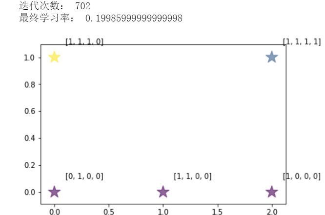
import numpy as np
import matplotlib.pyplot as plt
import math
import csv

# 向量归一化,转化为对应单位向量,这样计算欧几里得距离就
# 可以转化为计算向量的点积(二维平面中,单位向量点积就是
# cos theta),点积越大距离越近
def normalize(vector):
    return vector / np.linalg.norm(vector)

class Som:
    def initialize(self, model, dimension):
        self.nodes = []
        # 初始化节点
        for i in range(model[0]):
            temp = []
            for j in range(model[1]):
                vector = np.random.randn(dimension) # 每个节点都包含一个维度和输入向量维度相同的向量
                vector = normalize(vector) # 归一化
                temp.append(vector)
            self.nodes.append(temp)
        self.model = model # 便于遍历节点

    def best_matching_unit(self, vector):
        result = [0, 0] # 返回优胜节点坐标
        max = -10000

        for i in range(self.model[0]):
            for j in range(self.model[1]):
                temp = self.nodes[i][j].dot(vector)
                if temp > max:
                    max = temp
                    result[0], result[1] = i, j
        return result

    def get_r_p(self, N): # 根据距离优胜节点的距离变化的值
        return 1.0 / math.exp(N)

    def neighbor(self, pos, table):
        result = []
        x = pos[0]
        y = pos[1]

        if x - 1 >= 0:
            if not table[x - 1][y]:
                result.append([x - 1, y])
                table[x - 1][y] = True

        if x + 1 < self.model[0]:
            if not table[x + 1][y]:
                result.append([x + 1, y])
                table[x + 1][y] = True

        if y - 1 >= 0:
            if not table[x][y - 1]:
                result.append([x, y - 1])
                table[x][y - 1] = True

        if y + 1 < self.model[1]:
            if not table[x][y + 1]:
                result.append([x, y + 1])
                table[x][y + 1] = True

        return result

    def get_neighbor(self, BMU, r): # 获取邻居节点,返回值为[[距离为1坐标集合..], [距离为2坐标集合..], [...], ...]
        result = []

        if r > 0:
            table = [] # 记录已经存入的结点
            for i in range(self.model[0]):
                table.append([False] * self.model[1])
            table[BMU[0]][BMU[1]] = True
            # print("table=", table)

            neighbors = self.neighbor(BMU, table); # 距离为1的节点
            result.append(neighbors)
            for i in range(r - 1):
                temp = []
                for x in neighbors:
                    temp += self.neighbor(x, table)
                neighbors = temp  # 距离为2+i的结点
                result.append(neighbors)

        return result

    def update_nodes(self, BMU, example, r, eta): # 参数:优胜节点坐标,输入向量,优胜领域半径,学习率
        # print("r, eta=", r, eta)
        # print("before update=", self.nodes)
        w = self.nodes[BMU[0]][BMU[1]]
        w += eta * self.get_r_p(0) * (example - w) # 更新优胜节点
        self.nodes[BMU[0]][BMU[1]] = normalize(w)

        neighbors = self.get_neighbor(BMU, r);
        # print("neighbors=", neighbors)
        for i in range(len(neighbors)):
            for pos in neighbors[i]: # 更新距离为i+1的节点
                w = self.nodes[pos[0]][pos[1]]
                w += eta * self.get_r_p(i + 1) * (example - w)
                self.nodes[pos[0]][pos[1]] = normalize(w)

        # print("after update=", self.nodes)

    def eta(self, t): # 参数:当前迭代次数,隐含参数:最大迭代次数,学习率初始值
        if t <= self.MAX_ITERATION / 10: # 前1/10次迭代学习率线性下降到1/20
            return self.init_eta - t * self.k1
        else: # 后9/10次迭代学习率线性下降到0
            return self.init_eta / 20 - (t - self.MAX_ITERATION / 10) * self.k2

    def get_r(self, t): # 优胜邻域随着迭代次数变小
        return int(self.init_r * (1 - t / self.MAX_ITERATION)) # 向下取整

    def train(self, get_batch, MAX_ITERATION, init_eta, MIN_ETA, init_r): # 参数:获取每次迭代所需样本的函数,最大迭代次数,学习率初始值,最小学习率,优胜领域初始值
        self.MAX_ITERATION = MAX_ITERATION
        self.init_eta = init_eta # 学习率初始值
        self.k1 = (19/20 * self.init_eta) / (1/10 * self.MAX_ITERATION) # 学习率线性下降斜率1
        self.k2 = (1/20 * self.init_eta) / (9/10 * self.MAX_ITERATION) # 学习率线性下降斜率2
        self.init_r = init_r
        count = 0
        while count < MAX_ITERATION and self.eta(count) > MIN_ETA:
            batch = get_batch()
            # print(">>>>>>>>>>>>>>>>>count=", count)
            # print("batch=", batch)
            for example in batch:
                # print("example=", example)
                BMU = self.best_matching_unit(example)
                # print("BMU=",BMU)
                self.update_nodes(BMU, example, self.get_r(count), self.eta(count))
            count = count + 1
        print("迭代次数:", count)
        print("最终学习率:", self.eta(count))

    def mapping(self, vector):
        vector = normalize(vector)
        return self.best_matching_unit(vector) # 返回优胜节点坐标

data = [[1, 0, 0, 0], [1, 1, 0, 0], [1, 1, 1, 0], [0, 1, 0, 0], [1, 1, 1, 1]]
features = np.array(list(map(normalize, data))) # 归一化

def full_batch():
    return features

som = Som()
som.initialize([3, 2], 4)

def testModel():
    result = list(map(som.mapping, features))

    count_pos = {}
    for pos in result:
        if result.count(pos) >= 1:
            count_pos[str(pos[0]) + ',' + str(pos[1])] = result.count(pos)

    x = np.array(list(map(lambda x: x[0], result)));
    y = np.array(list(map(lambda x: x[1], result)));
    size = np.array(list(map(lambda x: count_pos[str(x[0]) + ',' + str(x[1])], result)));
    color = np.arctan2(y, x)

    plt.scatter(x, y, s=size * 300, c=color,alpha=0.6, marker='*')
    for i in range(len(x)): # 打上标签
        plt.annotate(str(data[i]), xy = (x[i], y[i]), xytext = (x[i]+0.1, y[i]+0.1))
    plt.show()

som.train(full_batch, 10000, 0.6, 0.2, 3)
testModel()

 浙公网安备 33010602011771号