seaborn绘图（kaggle）

jupyter notebook绘图初始化代码

import pandas as pd
pd.plotting.register_matplotlib_converters()
import matplotlib.pyplot as plt
%matplotlib inline
import seaborn as sns
print("Setup Complete")

不同类型的绘图

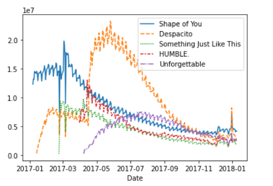
1. sns.lineplot()
   https://www.kaggle.com/code/alexisbcook/line-charts

sns.lineplot(data=spotify_data)

2. sns.barplot()
   https://www.kaggle.com/code/alexisbcook/bar-charts-and-heatmaps

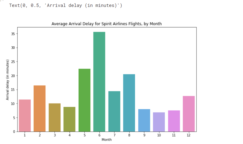
# Set the width and height of the figure
plt.figure(figsize=(10,6))

# Add title
plt.title("Average Arrival Delay for Spirit Airlines Flights, by Month")

# Bar chart showing average arrival delay for Spirit Airlines flights by month
sns.barplot(x=flight_data.index, y=flight_data['NK'])

# Add label for vertical axis
plt.ylabel("Arrival delay (in minutes)")

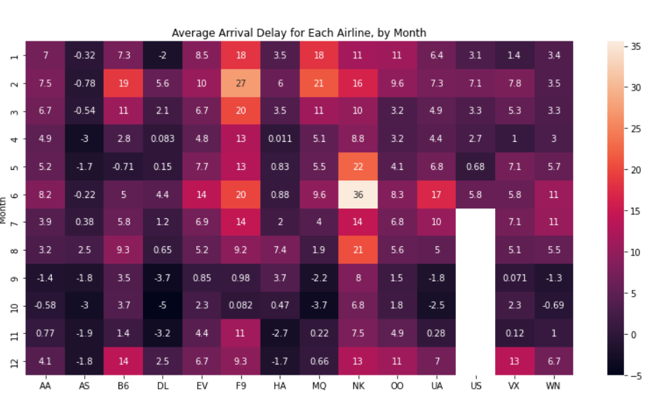
3. sns.heatmap()

# Set the width and height of the figure
plt.figure(figsize=(14,7))

# Add title
plt.title("Average Arrival Delay for Each Airline, by Month")

# Heatmap showing average arrival delay for each airline by month
sns.heatmap(data=flight_data, annot=True)

# Add label for horizontal axis
plt.xlabel("Airline")

annot=True 在图标内显示数值
https://www.kaggle.com/code/alexisbcook/bar-charts-and-heatmaps

4. sns.scatterplot()
https://www.kaggle.com/code/alexisbcook/scatter-plots

sns.scatterplot(x=insurance_data['bmi'], y=insurance_data['charges'])

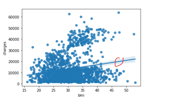
5. sns.regplot()

sns.regplot(x=insurance_data['bmi'], y=insurance_data['charges'])

在原图上添加了一条回归线

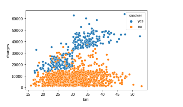
sns.scatterplot(x=insurance_data['bmi'], y=insurance_data['charges'], hue=insurance_data['smoker'])

多添加了hue参数，用于类别划分

6. sns.lmplot()

sns.lmplot(x="bmi", y="charges", hue="smoker", data=insurance_data)

每个类别都绘制了一条回归线


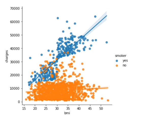
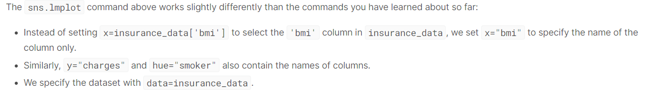
翻译：sns.lmplot的绘图方式与之前的几个不大一样，之前的都是x=data['列名'],y=data['列名'],这个则是x='col_name',y='col_name',data=data
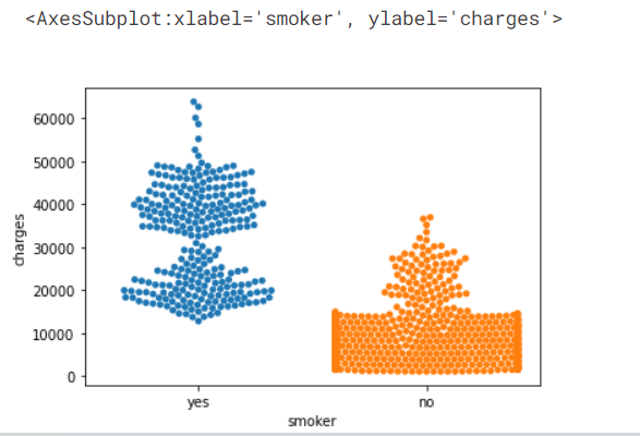
7. sns.swarmplot()
https://www.kaggle.com/code/alexisbcook/scatter-plots

sns.swarmplot(x=insurance_data['smoker'],
              y=insurance_data['charges'])

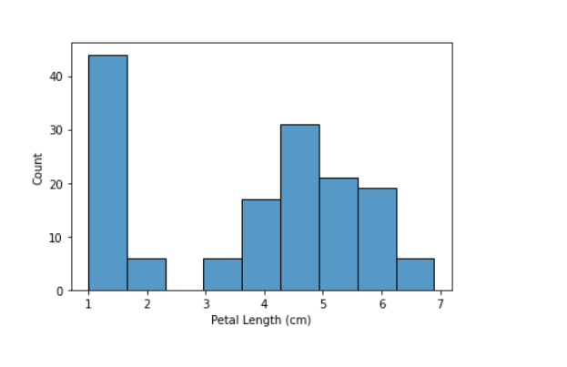
8. sns.histplot()
https://www.kaggle.com/code/alexisbcook/distributions

# Histogram 
sns.histplot(iris_data['Petal Length (cm)'])

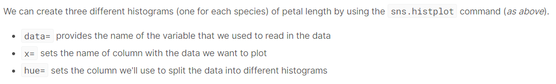
上点颜色

# Histograms for each species
sns.histplot(data=iris_data, x='Petal Length (cm)', hue='Species')

# Add title
plt.title("Histogram of Petal Lengths, by Species")

一些解释

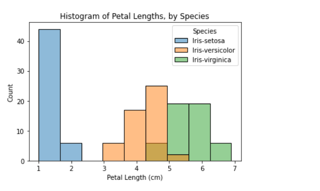
9，10密度图
9. sns.kdeplot()
https://www.kaggle.com/code/alexisbcook/distributions
The next type of plot is a kernel density estimate (KDE)plot. In case you're not familiar with KDE plots, you can think of it as a smoothed histogram.
翻译：如果不熟悉KDE图，可以把KDE图近似地理解成直方图的平滑曲线版

# KDE plot 
sns.kdeplot(data=iris_data['Petal Length (cm)'], shade=True)

shade=True 表示将曲线下方的区域上色

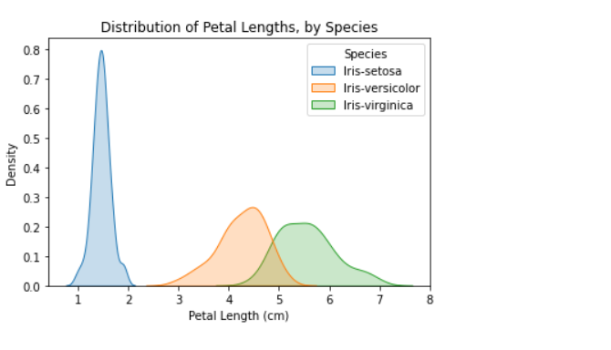
上点颜色

# KDE plots for each species
sns.kdeplot(data=iris_data, x='Petal Length (cm)', hue='Species', shade=True)

# Add title
plt.title("Distribution of Petal Lengths, by Species")

10. sns.jointplot()
    a two-dimensional (2D) KDE plot

# 2D KDE plot
sns.jointplot(x=iris_data['Petal Length (cm)'], y=iris_data['Sepal Width (cm)'], kind="kde")

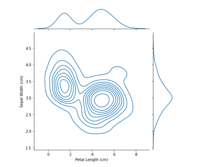
一些对上图的解释：
Note that in addition to the 2D KDE plot in the center,

• the curve at the top of the figure is a KDE plot for the data on the x-axis (in this case, iris_data['Petal Length (cm)']), and
• the curve on the right of the figure is a KDE plot for the data on the y-axis (in this case, iris_data['Sepal Width (cm)']).

改变画布的风格主题

只需要一行代码： sns.set_style("xxx")
可选参数有5个，分别为:
'darkgrid','whitegrid','dark','white','ticks'

# Change the style of the figure to the "dark" theme
sns.set_style("dark")

# Line chart 
plt.figure(figsize=(12,6))
sns.lineplot(data=spotify_data)