7. The Singular Value Decomposition(SVD)

7.1 Singular values and Singular vectors

The SVD separates any matrix into simple pieces.

A is any m by n matrix, square or rectangular, Its rank is r.

Choices from the SVD

\[AA^Tu_i = \sigma_i^{2}u_i \\ A^TAv_i = \sigma_i^{2}v_i \\ Av_i = \sigma_i u_i \]

\(u_i\)— the left singular vectors (unit eigenvectors of \(AA^T\))

\(v_i\)— the right singular vectors (unit eigenvectors of \(A^TA\))

\(\sigma_i\)— singular values (square roots of the equal eigenvalues of \(AA^T\) and \(A^TA\))

The rank of A is equal to numbers of \(\sigma _i\)

example:

\[A = \left [ \begin{matrix} 1&0 \\ 1&1 \end{matrix}\right] \\ \Downarrow \\ AA^T = \left [ \begin{matrix} 1&0 \\ 1&1 \end{matrix}\right] \left [ \begin{matrix} 1&1 \\ 0&1 \end{matrix}\right] =\left [ \begin{matrix} 1&1 \\ 1&2 \end{matrix}\right] \\ A^TA = \left [ \begin{matrix} 1&1 \\ 0&1 \end{matrix}\right] \left [ \begin{matrix} 1&0 \\ 1&1 \end{matrix}\right] =\left [ \begin{matrix} 2&1 \\ 1&1 \end{matrix}\right] \\ \Downarrow \\ det(AA^T - I) = 0 \ \quad \ det(A^TA - I) = 0 \\ \lambda_1 = \frac{3+\sqrt{5}}{2} , \sigma_1=\frac{1+\sqrt{5}}{2}, u_1= \frac{1}{\sqrt{1+\sigma_1^2}}\left [ \begin{matrix} 1 \\ \sigma_1 \end{matrix}\right], v_1= \frac{1}{\sqrt{1+\sigma_1^2}}\left [ \begin{matrix} \sigma_1 \\ 1 \end{matrix}\right] \\ \lambda_2 = \frac{3-\sqrt{5}}{2} , \sigma_1=\frac{1-\sqrt{5}}{2}, u_2= \frac{1}{\sqrt{1+\sigma_2^2}}\left [ \begin{matrix} \sigma_1 \\ -1 \end{matrix}\right], v_2= \frac{1}{\sqrt{1+\sigma_2^2}}\left [ \begin{matrix} 1 \\ -\sigma_1 \end{matrix}\right]\\ \Downarrow \\ A = \left [ \begin{matrix} u_1&u_2 \end{matrix}\right] \left [ \begin{matrix} \sigma_1&\\&\sigma_2 \end{matrix}\right] \left [ \begin{matrix} v_1^T\\v_2^T \end{matrix}\right] \\ A\left [ \begin{matrix} v_1&v_2 \end{matrix}\right] = \left [ \begin{matrix} u_1&u_2 \end{matrix}\right] \left [ \begin{matrix} \sigma_1&\\&\sigma_2 \end{matrix}\right] \]

7.2 Bases and Matrices in the SVD

Keys:

1. The SVD produces orthonormal basis of \(u's\) and $ v's$ for the four fundamental subspaces.

   • \(u_1,u_2,...,u_r\) is an orthonormal basis of the column space. (\(R^m\))
   • \(u_{r+1},...,u_{m}\) is an orthonormal basis of the left nullspace. (\(R^m\))
   • \(v_1,v_2,...,v_r\) is an orthonormal basis of the row space. (\(R^n\))
   • \(v_{r+1},...,u_{n}\) is an orthonormal basis of the nullspace.(\(R^n\))

2. Using those basis, A can be diagonalized :

   Reduced SVD: only with bases for the row space and column space.

   \[A = U_r \Sigma_r V_r^T \\ U = \left [ \begin{matrix} u_1&\cdots&u_r\\ \end{matrix}\right] , \Sigma_r = \left [ \begin{matrix} \sigma_1&&\\&\ddots&\\&&\sigma_r \end{matrix}\right], V_r^T=\left [ \begin{matrix} v_1\\ \vdots \\ v_r \end{matrix}\right] \\ \Downarrow \\ A = \left [ \begin{matrix} u_1&\cdots&u_r\\ \end{matrix}\right] \left [ \begin{matrix} \sigma_1&&\\&\ddots&\\&&\sigma_r \end{matrix}\right] \left [ \begin{matrix} v_1\\ \vdots \\ v_r \end{matrix}\right] \\ = u_1\sigma_1v_{1}^T + u_2\sigma_2v_{2}^T + \cdots + u_r\sigma_rv_r^T \]

   Full SVD: include four subspaces.

   \[A = U \Sigma V^T \\ U = \left [ \begin{matrix} u_1&\cdots&u_r&\cdots&u_n\\ \end{matrix}\right] , \Sigma_r = \left [ \begin{matrix} \sigma_1&&\\&\ddots&\\&&\sigma_r \\ &&&\ddots \\ &&&&\sigma_n \end{matrix}\right], V^T=\left [ \begin{matrix} v_1\\ \vdots \\ v_r \\ \vdots \\ v_m \end{matrix}\right] \\ \Downarrow \\ A = \left [ \begin{matrix} u_1&\cdots&u_r&\cdots&u_n\\ \end{matrix}\right] \left [ \begin{matrix} \sigma_1&&\\&\ddots&\\&&\sigma_r \\ &&&\ddots \\ &&&&\sigma_n \end{matrix}\right] \left [ \begin{matrix} v_1\\ \vdots \\ v_r \\ \vdots \\ v_m \end{matrix}\right] \\ = u_1\sigma_1v_{1}^T + u_2\sigma_2v_{2}^T + \cdots + u_r\sigma_rv_r^T\cdots + u_n\sigma_n v_n^{T} + \cdots + u_m\sigma_mv_m^T \]

   example: \(A=\left [ \begin{matrix} 3&0 \\ 4&5 \end{matrix}\right]\), r=2

   \[A^TA =\left [ \begin{matrix} 25&20 \\ 20&25 \end{matrix}\right], AA^T =\left [ \begin{matrix} 9&12 \\ 12&41 \end{matrix}\right] \\ \lambda_1 = 45, \sigma_1 = \sqrt{45}, v_1 = \frac{1}{\sqrt{2}} \left [ \begin{matrix} 1 \\ 1 \end{matrix}\right], u_1 = \frac{1}{\sqrt{10}} \left [ \begin{matrix} 1 \\ 3 \end{matrix}\right]\\ \lambda_2 = 5, \sigma_2 = \sqrt{5} , v_2 = \frac{1}{\sqrt{2}} \left [ \begin{matrix} -1 \\ 1 \end{matrix}\right], u_2 = \frac{1}{\sqrt{10}} \left [ \begin{matrix} -3 \\ 1 \end{matrix}\right]\\ \Downarrow \\ U = \frac{1}{\sqrt{10}} \left [ \begin{matrix} 1&-3 \\ 3&1 \end{matrix}\right], \Sigma = \left [ \begin{matrix} \sqrt{45}& \\ &\sqrt{5} \end{matrix}\right], V = \frac{1}{\sqrt{2}} \left [ \begin{matrix} 1&-1 \\ 1&1 \end{matrix}\right] \]

7.3 The geometry of the SVD

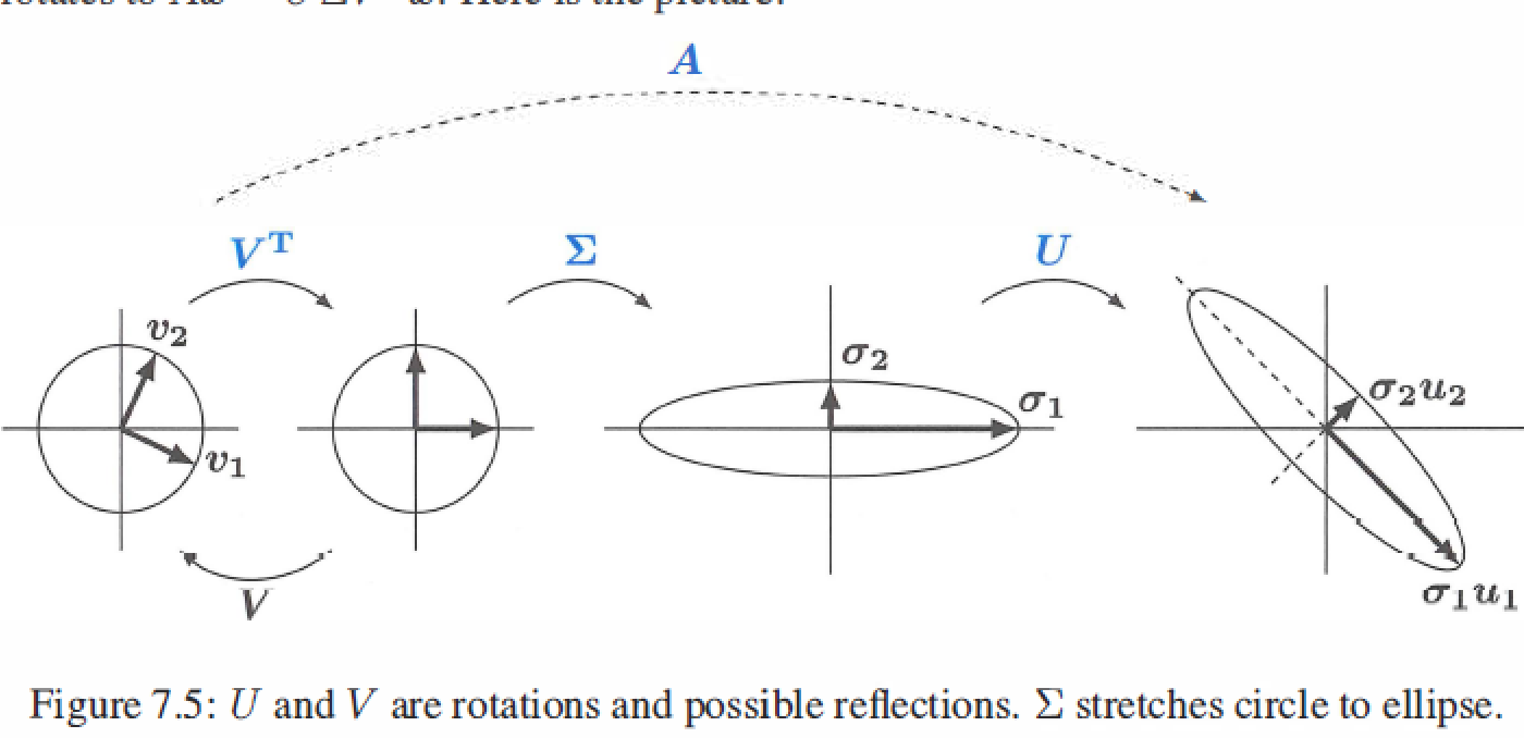
1. \(A = U\Sigma V^T\) factors into (rotation)(stretching)(rotation), the geometry shows how A transforms vectors x on a circle to vectors Ax on an ellipse.

2. Polar decomposition factors A into QS : rotation \(Q=UV^T\) times streching \(S=V \Sigma V^T\).

   \[V^TV = I \\ A = U\Sigma V^T = (UV^T)(V\Sigma V^T) = (Q)(S) \]

   Q is orthogonal and inclues both rotations U and \(V^T\), S is symmetric positive semidefinite and gives the stretching directions.

   If A is invertible, S is positive definite.

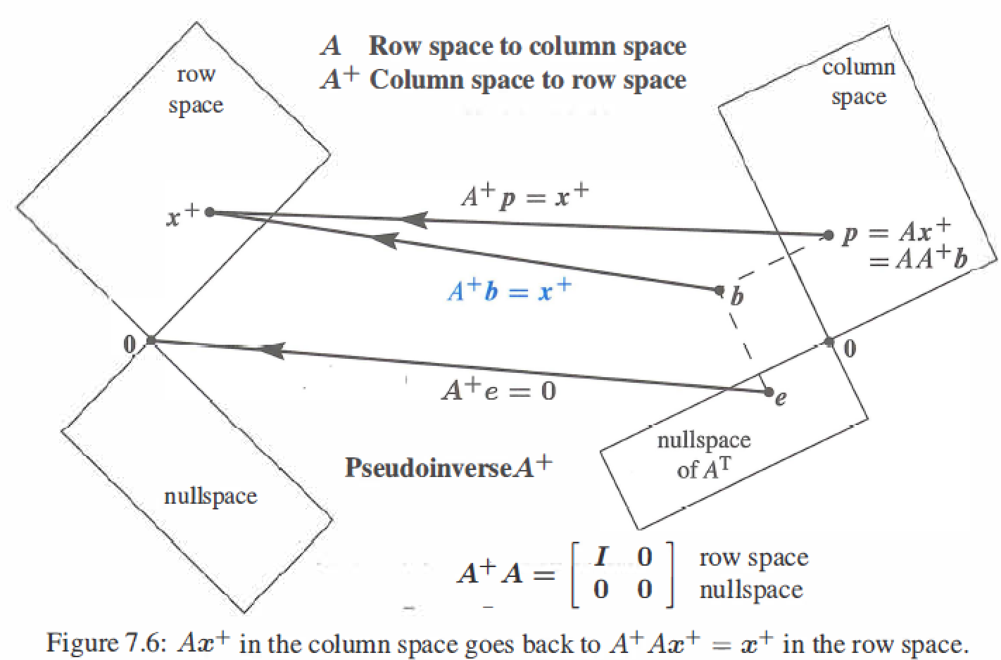
3. The Pseudoinverse \(A^{+}: AA^{+}=I\)

   • \(Av_i=\sigma_iu_i\) : A multiplies \(v_i\) in the row space of A to give \(\sigma_i u_i\) in the column space of A.

   • If \(A^{-1}\) exists, \(A^{-1}u_i=\frac{v_i}{\sigma}\) : \(A^{-1}\) multiplies \(u_i\) in the row space of \(A^{-1}\) to give \(\sigma_i u_i\) in the column space of \(A^{-1}\), \(1/\sigma_i\) is singular values of \(A^{-1}\).

   • Pseudoinverse of A: if \(A^{-1}\) exists, then \(A^{+}\) is the same as \(A^{-1}\)

     \[A^{+} = V \Sigma^{+}U^{T} = \left [ \begin{matrix} v_1&\cdots&v_r&\cdots&v_n\\ \end{matrix}\right] \left [ \begin{matrix} \sigma_1^{-1}&&\\&\ddots&\\&&\sigma_r^{-1} \\ &&&\ddots \\ &&&&\sigma_n^{-1} \end{matrix}\right] \left [ \begin{matrix} u_1\\ \vdots \\ u_r \\ \vdots \\ u_m \end{matrix}\right] \\ \]

7.4 Principal Component Analysis ( PCA by the SVD)

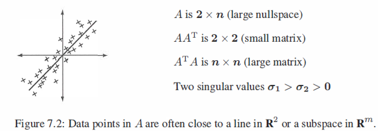
PCA gives a way to understand a data plot in dimension m, applications mostly are human genetics \ face recognition\ finance \ model order reduction (computation) .

The sample covariance matrix \(S=AA^T/(n-1)\)

The crucial connection to linear algebra is in the singular values and singular vectors of A, which comes from the eigenvalues \(\lambda=\sigma^2\) and the eigenvectors u of the sample covariance matrix \(S=AA^T/(n-1)\)

1. The total variance in the data is the sum of all eigenvalues and of sample variances \(s^2\) :

   \[T = \sigma_1^2 + \cdots + \sigma_m^2 = s_1^2 + \cdots + s_m^2 = trace(diagonal \ \ sum) \]

2. The first eigenvector \(u_1\) of S points in the most significant direction of the data.That direction accounts for a fraction \(\sigma_1^2/T\) of the total variance.

3. The next eigenvectors \(u_2\) (orthogonal to \(u_1\)) accounts for a small fraction \(\sigma_2^2/T\).

4. Stop when those fractions are small. You have the R directions that explain most of the data.The n data points are very near an R-dimensional subspace with basis \(u_1, \cdots, u_R\), which are the principal components.

5. R is the "effective rank" of A. The true rank r is probably m or n : full rank matrix.

example: \(A = \left[ \begin{matrix} 3&-4&7&-1&-4&-3 \\ 7&-6&8&-1&-1&-7 \end{matrix} \right]\) has sample covariance \(S=AA^T/5 = \left [ \begin{matrix} 20&25 \\ 25&40 \end{matrix}\right]\)

The eigenvalues of S are 57 and 3，so the first rank one piece \(\sqrt{57}u_1v_1^T\) is much larger than the second piece \(\sqrt{3}u_2v_2^T\).

The leading eigenvector \(u_1 = (0.6,0.8)\) shows the direction that you see in the scatter graph.

The SVD of A (centered data) shows the dominant direction in the scatter plot.

The second eigenvector \(u_2\) is perpendicular to \(u_1\). The second singular value \(\sigma_2=\sqrt{3}\) measures the spread across the dominant line.