4. Orthogonality

4.1 Orthogonal Vectors and Suspaces

• Orthogonal vectors have \(v^Tw=0\)，and \(||v||^2 + ||w||^2 = ||v+w||^2 = ||v-w||^2\).

• Subspaces \(V\) and \(W\) are orthogonal when \(v^Tw = 0\) for every \(v\) in V and every \(w\) in W.

• Four Subspaces Relations:

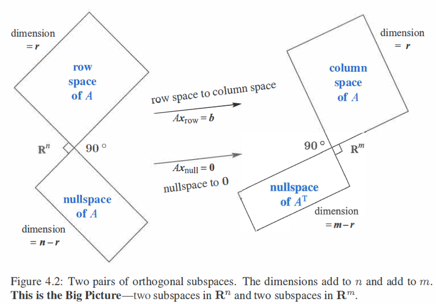
  • Every vector x in the nullspace is perpendicular to every row of A, because \(Ax=0\).The nullspace N(A) and the row space \(C(A^T)\) are orthogonal subspaces of \(R^n\). \(N(A) \bot C(A^T)\)

    \[Ax = \left[ \begin{matrix} &row_1& \\ &\vdots \\ &row_m \end{matrix} \right] \left[ \begin{matrix} && \\ &x \\ && \end{matrix} \right] = \left[ \begin{matrix} &0& \\ &\vdots \\ &0 \end{matrix} \right] \]

  • Every vector y in the nullspace of \(A^T\) is perpendicular to every column of A, because \(A^Ty=0\).The left nullspace \(N(A^T)\) and the column space \(C(A)\) are orthogonal subspaces of \(R^m\). \(N(A^T) \bot C(A)\)

    \[A^Ty = \left[ \begin{matrix} &(column_1)^T& \\ &\vdots \\ &(column_m)^T \end{matrix} \right] \left[ \begin{matrix} && \\ &y \\ && \end{matrix} \right] = \left[ \begin{matrix} &0& \\ &\vdots \\ &0 \end{matrix} \right] \]

  • The nullspace N(A) and the row space \(C(A^T)\) are orthogonal complements, with dimensions (n-r) + r = n. Similarly \(N(A^T)\) and C(A) are orthogonal complements with (m-r) + r = m.

4.2 Projection

When b is not in the columns space C(A)，then Ax = b is unsolvable，so find the projection p of b onto C(A)，make \(A\hat{x} = p\) is solvable.

Three Steps:

1. Find \(\hat{x}\)
2. Find p
3. Find project matrix P

Projection Onto a Line

A line goes through the origin in the direction of \(a=(a_1, a_2,...,a_m)\).

Along that line, we want the point \(p\) closest to \(b=(b_1,b_2,...,b_m)\).

The key to projection is orthogonality : The line from b to p is perpendicular to the vector a.

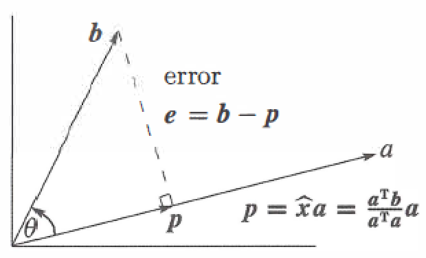
Projecting b onto a with error \(e=b-\hat{x}a\) :

\[a \cdot(b-\hat{x}a) = a^T(b-\hat{x}a)=0 \\ \Downarrow \\ \hat{x} = \frac{a \cdot b}{a \cdot a} = \frac{a^T b}{a^T a} \\ \Downarrow \\ p = a \hat{x} =a\frac{a^T b}{a^T a} = Pb \\ \Downarrow \\ P = \frac{aa^T}{a^Ta} \\ \]

\(P=P^T\) (P is symmetric) , \(P^2=P\)

Projection Onto a Subspace

Start with n independent vectors \(A=(a_1,...,a_n)\) in \(R^m\), find the combination \(p=\hat{x}a_1 + \hat{x}a_2 +...+\hat{x_n}a_n\) closest to a givent vector b.

\[A^T(b-A\hat{x}) = \left[ \begin{matrix} -&a_1^T&- \\ &\vdots \\ -&a_n^T&- \end{matrix} \right] \left[ \begin{matrix} && \\ &b-A\hat{x} \\ && \end{matrix} \right] = \left[ \begin{matrix} &0& \\ &\vdots \\ &0 \end{matrix} \right] \\ \Downarrow \\ A^T(b-A\hat{x}) = 0 \ \ 或 \ \ \ A^TA\hat{x} = A^Tb \\ \Downarrow A^TA \ \ invertible\\ p=A\hat{x} = A(A^TA)^{-1}A^Tb \\ \Downarrow \\ P=A(A^TA)^{-1}A^T \]

\(P=P^T\) (P is symmetric) , \(P^2=P\)

4.3 Least Squares Approximations

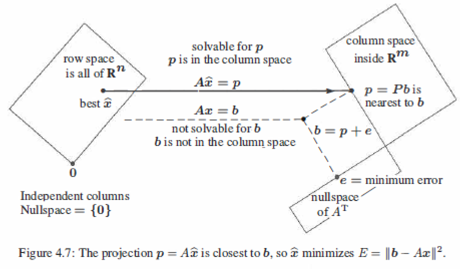
When b is outside the column space of A, that \(Ax=b\) has no solution. Find the length of \(e=b-Ax\) as small as possible, get a \(\hat{x}\) is a least squares solution.

If A has independent columns, then \(A^TA\) is invertible.

proof :

\[A^TAx = 0 \\ \Downarrow \\ x^TA^TAx = 0 \\ \Downarrow \\ (Ax)^TAx =0 \\ \Downarrow \\ Ax =0 \\ \ A \ \ is \ \ independent \\ \Downarrow \\ x=0 \]

so \(N(A^TA)\) has only zero vector, \(A^TA\) is invertible.

Linear algebra method (projection method)

Sovling \(A^TA\hat{x} = A^Tb\) gives the projection \(p=A\hat{x}\) of b onto the column space of A.

\[Ax=b \ \ (unsolvable) \\ b = p+e \\ \Downarrow \\ A\hat{x} = p \ \ (solvable) \\ \Downarrow \\ \hat{x} = (A^TA)^{-1}A^Tb \]

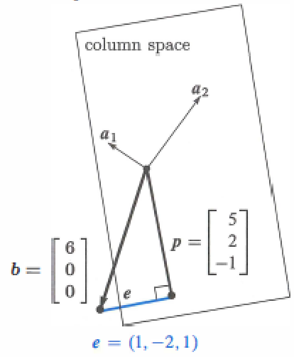
example: \(A = \left[ \begin{matrix} 1&1 \\ 1&2 \\ 1&3 \end{matrix} \right], x= \left[ \begin{matrix} C \\ D \end{matrix} \right], b=\left[ \begin{matrix} 1 \\ 2 \\ 2 \end{matrix} \right], Ax=b\) is unsolvable.

\[A^TA\hat{x} = A^Tb \\ \Downarrow \\ A^TA = \left[ \begin{matrix} 1&1&1 \\ 1&2&3 \end{matrix} \right] \left[ \begin{matrix} 1&1 \\ 1&2 \\ 1&3 \end{matrix} \right] = \left[ \begin{matrix} 3&6 \\ 6&14 \end{matrix} \right] \\ A^Tb = \left[ \begin{matrix} 1&1&1 \\ 1&2&3 \end{matrix} \right] \left[ \begin{matrix} 1 \\ 2 \\ 2 \end{matrix} \right] = \left[ \begin{matrix} 5 \\ 11 \end{matrix} \right] \\ \Downarrow \\ \left[ \begin{matrix} 3&6 \\ 6&14 \end{matrix} \right] \left[ \begin{matrix} C \\ D\\ \end{matrix} \right] = \left[ \begin{matrix} 5 \\ 11 \end{matrix} \right] \\ \Downarrow \\ C = 2/3 \ , \ D=1/2 \\ \Downarrow \\ \hat{x} = \left[ \begin{matrix} 2/3 \\ 1/2\end{matrix} \right] \\ \]

Calculus method

The least squares solution \(\hat{x}\) makes the sum of errors \(E = ||Ax - b||^2\) as small as possible.

\[E = e_1^2 + e_2^2 +...+e_n^2 \]

example: \(A = \left[ \begin{matrix} 1&1 \\ 1&2 \\ 1&3 \end{matrix} \right], x= \left[ \begin{matrix} C \\ D \end{matrix} \right], b=\left[ \begin{matrix} 1 \\ 2 \\ 2 \end{matrix} \right], Ax=b\) is unsolvable.

\[E = ||Ax - b||^2 = e_1^2 + e_2^2 +e_3^2 = (C +D \cdot 1 -1)^2 + (C +D \cdot 2 -2)^2 + (C +D \cdot 3 -2)^2 \\ \Downarrow \\ \part E / \part C = 0 \\ \part E / \part D = 0 \\ \Downarrow \\ C = 2/3 \ , \ D=1/2 \]

The Big Picture for Least Squares

4.4 Orthonormal Bases and Gram-Schmidt

• The columns \(q_1,q_2,...,q_n\) are orthonormal if \(q_i^Tq_j = \left \{ \begin{array}{rcl} 0 \ \ for \ \ i \neq j \\ 1 \ \ for \ \ i=j \end{array}\right\}, Q^TQ=I\).
• If Q is also square, the \(QQ^T=I\) and \(Q^T=Q^{-1}\), Q is an orthogonal matrix.
• The least squares solution to \(Qx = b\) is \(\hat{x} = Q^Tb\). Projection of b : \(p=QQ^Tb = Pb\).

Projection Using Orthonormal Bases: Q Repalces A

Orthogonal matrices are excellent and stable for computations.

Suppose the basis vectors are actually orthonormal, then \(A^TA\) simplifies to \(Q^TQ\), here is \(\hat{x} = Q^Tb\) and \(p=Q\hat{x}=QQ^Tb\).

\[\\ \ p = \left[ \begin{matrix} |&&| \\ q_1&\cdots&q_n \\ |&&| \end{matrix} \right] \left[ \begin{matrix} q_1^Tb \\ \vdots \\ q_n^Tb \end{matrix} \right] = q_1(q_1^Tb) + ... + q_n(q_n^Tb) \]

The Gram-Schmidt Process

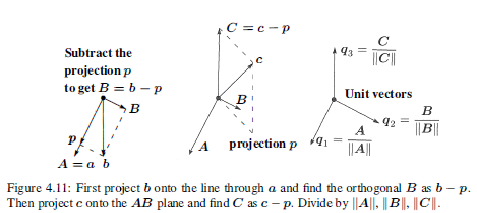
"Gram-Schmidt way" is to create orthonormal vectors.Take independent column vecotrs \(a_i\) to orthonormal \(q_i\).

From independent vectors \(a_1,...,a_n\)，Gram-Schmidt constructs orthonormal vectors \(q_1,...,q_n\).The matrices with these columns satisfy \(A=QR\). The \(R=Q^TA\) is upper triangular because later q's are orthoganal to a's.

Gram-Schmidt Process:

Subtract from every new vector its projections in the directions already set.

• First step : Chosing A=a and \(B = b-\frac{A^Tb}{A^TA}A\) -----> $A \bot B $
• Second step : \(C = c-\frac{A^Tc}{A^TA}A - \frac{B^Tc}{B^TB}B\) -----> $C \bot A \ \ C \bot B $
• Last step (orthonormal): \(q_1 = \frac{A}{||A||},q_2 = \frac{B}{||B||},q_3 = \frac{C}{||C||}\)

The \(q_1,q_2,q_3\) is the orthgonormal base. \(Q=\left[ \begin{matrix} && \\ q_1&q_2&q_3 \\ && \end{matrix} \right]\)

**The Factorization M = QR **：

Any m by n matrix M with independent columns can be factored into \(M=QR\).

\[M=QR=\left[ \begin{matrix} &&\\ q_1&q_2&q_3 \\ && \end{matrix} \right] \left[ \begin{matrix} q_1^Ta&q_1^Tb&q_1^Tc \\ &q_2^Tb&q_2^Tc \\ &&q_3^Tc \end{matrix} \right] \]

example:

Suppose the independent not-orthogonal vectors \(a,b,c\) are

\[a = \left[ \begin{matrix} 1 \\ -1 \\ 0\end{matrix} \right] \ and \ \ b = \left[ \begin{matrix} 2 \\ 0 \\ -2\end{matrix} \right] \ and \ \ c = \left[ \begin{matrix} 3 \\ -3 \\ 3\end{matrix} \right] \]

Then A=a has \(A^TA=2, A^Tb=2\)

First step : \(B=b-\frac{A^Tb}{A^TA}A = \left[ \begin{matrix} 1 \\ 1 \\ -2\end{matrix} \right]\)

Second step : \(C=c-\frac{A^Tc}{A^TA}A -\frac{B^Tc}{B^TB}B = \left[ \begin{matrix} 1 \\ 1 \\ 1\end{matrix} \right]\)

Last step : \(q_1 = \frac{A}{||A||}= \frac{1}{\sqrt{2}}\left[ \begin{matrix} 1 \\ -1 \\ 0\end{matrix} \right],q_2 = \frac{B}{||B||}=\frac{1}{\sqrt{6}}\left[ \begin{matrix} 1 \\ 1 \\ -2\end{matrix} \right],q_3 = \frac{C}{||C||}=\frac{1}{\sqrt{3}}\left[ \begin{matrix} 1 \\ 1 \\ 1\end{matrix} \right]\)

Factorization :

\[M =\left[ \begin{matrix} 1&2&3 \\ -1&0&-3 \\ 0&-2&3 \end{matrix} \right] = \left[ \begin{matrix} 1/\sqrt{2}&1/\sqrt{6}&1/\sqrt{3} \\ -1/\sqrt{2}&1/\sqrt{6}&1/\sqrt{3} \\ 0&-2/\sqrt{6}&1/\sqrt{3} \end{matrix} \right] \left[ \begin{matrix} \sqrt{2}&\sqrt{2}&\sqrt{18} \\ 0&\sqrt{6}&-\sqrt{6} \\ 0&0&\sqrt{3} \end{matrix} \right] = QR \]

Least squares

Instead of solving \(Ax=b\), which is impossible, we finally solve \(R\hat{x}=Q^Tb\) by back substitution which is very fast.

\[A^TA\hat{x}=A^Tb \\ A^TA =(QR)^TQR = R^TQ^TQR=R^TR \\ \Downarrow \\ R^TR\hat{x} =R^TQ^Tb \quad or \quad R\hat{x} =Q^Tb \quad or \quad \hat{x} =R^{-1}Q^Tb \\ \]