随笔 - 54 文章 - 0 评论 - 45 阅读 - 45万

6.OpenCV 之平面单应性2021-04-02

7.OpenCV 之图像几何变换2021-03-25 8.OpenCV 之角点检测2021-03-11 9.OpenCV 之编译配置 4.6.02016-08-14 10.OpenCV 之 Mat 类2017-08-08 11.OpenCV 之网络摄像头2017-07-12 12.OpenCV 之神经网络 (一)2017-06-27 13.OpenCV 之图像边缘检测2016-06-05 14.OpenCV 之基本绘图2020-04-21 15.OpenCV 之支持向量机 (一)2016-07-30

上篇 OpenCV 之图像几何变换介绍了等距、相似和仿射变换，本篇侧重投影变换的平面单应性、OpenCV相关函数、应用实例等。

1 投影变换

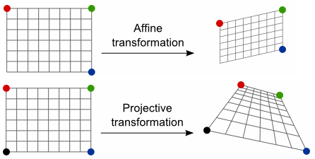
投影变换 (Projective Transformation)，是仿射变换的一般化，二者区别如下：

1.1 平面单应性

假定平面 $P^{2}$ 与 $Q^{2}$ 之间，存在映射，使得 $P^{2}$ 内任意点 $(x_p, y_q)$ ，满足下式：

$\quad \begin{bmatrix} x_q \\ y_q \\ 1 \end{bmatrix} = \begin{bmatrix} h_{11} & h_{12} & h_{13} \\ h_{21} & h_{22} & h_{23} \\ h_{31} & h_{32} & h_{33} \end{bmatrix} \begin{bmatrix} x_p \\ y_p \\ 1 \end{bmatrix}$

当 $H_{3 \times 3}$ 非奇异时， $P^{2}$ 与 $Q^{2}$ 之间的映射即为 2D 投影变换，也称， $H_{3 \times 3}$ 则为单应性矩阵

例如：在相机标定中，如果选用平面标定板，则物平面和像平面之间，就是一种典型的平面单应性映射

1.2 单应性矩阵

$H_{3 \times 3}$ 有 9 个未知数，但实际只有 8 个自由度 (DoF)，其归一化有两种方法：

法一，令 $h_{33}=1$ ；法二，加单位向量限制 $h_{11}^2+h_{12}^2+h_{13}^2+h_{21}^2+h_{22}^2+h_{23}^2+h_{31}^2+h_{32}^2+h_{33}^2=1$

下面接着法一，继续推导公式：

$\quad x' = \dfrac{h_{11}x + h_{12}y + h_{13}}{h_{31}x + h_{32}y + 1}$

$\quad y' = \dfrac{h_{21}x + h_{22}y + h_{23}}{h_{31}x + h_{32}y + 1}$

整理得：

$\quad x \cdot h_{11} + y \cdot h_{12} + h_{13} - xx' \cdot h_{31} - yx' \cdot h_{32} = x'$

$\quad x \cdot h_{21} + y \cdot h_{22} + h_{23} - xy' \cdot h_{31} - yy' \cdot h_{32} = y'$

一组对应特征点 $(x, y)$ -> $(x', y')$ 可构造 2 个方程，要求解 8 个未知数 (归一化后的)，则需要 8 个方程，4 组对应特征点

$\quad \begin{bmatrix} x_{1} & y_{1} & 1 &0 &0&0 & -x_{1}x'_{1} & -y_{1}x'_{1} \\ 0&0&0& x_{1} & y_{1} &1& -x_{1}y'_{1} & -y_{1}y'_{1} \\ x_{2} & y_{2} & 1 &0 &0&0 & -x_{2}x'_{2} & -y_{2}x'_{2} \\ 0&0&0& x_{2} & y_{2} &1& -x_{2}y'_{2} & -y_{2}y'_{2} \\ x_{3} & y_{3} & 1 &0 &0&0 & -x_{3}x'_{3} & -y_{3}x'_{3} \\ 0&0&0& x_{3} & y_{3} &1& -x_{3}y'_{3} & -y_{3}y'_{3} \\ x_{4} & y_{4} & 1 &0 &0&0 & -x_{4}x'_{4} & -y_{4}x'_{4} \\ 0&0&0& x_{4} & y_{4} &1& -x_{4}y'_{4} & -y_{4}y'_{4} \end{bmatrix} \begin{bmatrix} h_{11} \\ h_{12}\\h_{13}\\h_{21}\\h_{22}\\h_{23}\\h_{31}\\h_{32} \end{bmatrix} = \begin{bmatrix} x'_{1}\\y'_{1}\\x'_{2}\\y'_{2}\\x'_{3}\\y'_{3}\\x'_{4}\\y'_{4} \end{bmatrix}$

因此，求 $H$ 可转化为求解 $Ax=b$ ，参见 OpenCV 中 getPerspectiveTransform() 的源码实现

2 OpenCV 函数

2.1 投影变换矩阵

已知四组对应特征点坐标，带入 getPerspectiveTransform() 函数中，可求解 src 投影到 dst 的单应性矩阵 $H_{3 \times 3}$

Mat getPerspectiveTransform (
    const Point2f     src[],    // 原图像的四角顶点坐标
    const Point2f     dst[],    // 目标图像的四角顶点坐标
    int solveMethod = DECOMP_LU // solve() 的解法
)　　

该函数的源代码实现如下：构造8组方程，转化为 $Ax=b$ 的问题，调用 solve() 函数来求解

Mat getPerspectiveTransform(const Point2f src[], const Point2f dst[], int solveMethod)
{
    Mat M(3, 3, CV_64F), X(8, 1, CV_64F, M.ptr());
    double a[8][8], b[8];
    Mat A(8, 8, CV_64F, a), B(8, 1, CV_64F, b);
 
    for( int i = 0; i < 4; ++i )
    {
        a[i][0] = a[i+4][3] = src[i].x;
        a[i][1] = a[i+4][4] = src[i].y;
        a[i][2] = a[i+4][5] = 1;
        a[i][3] = a[i][4] = a[i][5] =
        a[i+4][0] = a[i+4][1] = a[i+4][2] = 0;
        a[i][6] = -src[i].x*dst[i].x;
        a[i][7] = -src[i].y*dst[i].x;
        a[i+4][6] = -src[i].x*dst[i].y;
        a[i+4][7] = -src[i].y*dst[i].y;
        b[i] = dst[i].x;
        b[i+4] = dst[i].y;
    }
 
    solve(A, B, X, solveMethod);
    M.ptr<double>()[8] = 1.;
 
    return M;
}　　

b) 多组对应特征点：对于两个平面之间的投影变换，求得对应的多组特征点后，带入 findHomography() 函数，便可得到 srcPoints 投影到 dstPoints 的 $H_{3 \times 3}$

Mat findHomography (
     InputArray      srcPoints,   // 原始平面特征点坐标，类型是 CV_32FC2 或 vector<Point2f> 
     InputArray      dstPoints,   // 目标平面特征点坐标，类型是 CV_32FC2 或 vector<Point2f> 
     int method = 0,              // 0--最小二乘法; RANSAC--基于ransac的方法
     double ransacReprojThreshold = 3, // 最大允许反投影误差
     OutputArray mask = noArray(),     // 
     const int maxIters = 2000,        // 最多迭代次数
     const double confidence = 0.995   // 置信水平
 )　　

2.2 投影变换图像

已知单应性矩阵 $H_{3 \times 3}$ ，将任意图像代入 warpPerspective() 中，便可得到经过 2D投影变换的目标图像

void warpPerspective (
    InputArray      src,  // 输入图像
    OutputArray     dst,  // 输出图象(大小 dsize，类型同 src)
    InputArray        M,  // 3x3 单应性矩阵
    Size          dsize,  // 输出图像的大小
    int     flags = INTER_LINEAR,         // 插值方法 
    int     borderMode = BORDER_CONSTANT, //
    const Scalar& borderValue = Scalar()  // 
)   　　

3 代码示例

3.1 透视校正

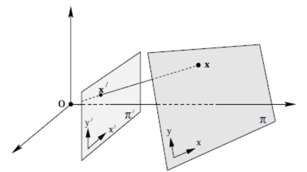
像平面 image1 和 image2 是相机在不同位置对同一物平面所成的像，这三个平面任选两个都互有平面单应性

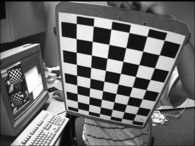
以相机标定为例，当人拿着棋盘格旋转不同角度时，可利用任意两个棋盘格间的单应性，将旋转不同角度的棋盘格，转换为统一角度

#include "opencv2/imgproc.hpp"
#include "opencv2/highgui.hpp"
#include "opencv2/calib3d.hpp"
 
using namespace cv;
 
Size kPatternSize = Size(9, 6);
 
int main()
{
    // 1) read image
    Mat src = imread("chessboard1.jpg");
    Mat dst = imread("chessboard2.jpg");
    if (src.empty() || dst.empty())
        return -1;
 
    // 2) find chessboard corners
    std::vector<Point2f> corners1, corners2;
    bool found1 = findChessboardCorners(src, kPatternSize, corners1);
    bool found2 = findChessboardCorners(dst, kPatternSize, corners2);
    if (!found1 || !found2)
        return -1;
 
    // 3) estimate H matrix
    Mat H = findHomography(corners1, corners2, RANSAC);
    // 4) 
    Mat src_warp;
    warpPerspective(src, src_warp, H, src.size());
 
    // 5) 
    imshow("src", src);
    imshow("dst", dst);
    imshow("src_warp", src_warp);
    waitKey();
}　　

结果如下：

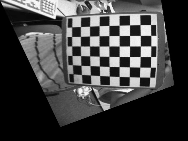
棋盘格倾斜棋盘格正对倾斜校正为正对

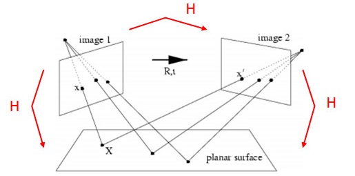
3.2 图像拼接

当相机围绕其投影轴，只做旋转运动时，所有的像素点可等效视为在一个无穷远的平面上，则单应性矩阵可由旋转变换 $R$ 和相机标定矩阵 $K$ 来表示

$\quad \normalsize s \begin{bmatrix} x' \\ y' \\1 \end{bmatrix} = \normalsize K \cdot \normalsize R \cdot \normalsize K^{-1} \begin{bmatrix} x \\ y \\ 1 \end{bmatrix}$

因此，如果已知相机的标定矩阵，以及旋转变换前后的位姿，可利用平面单应性，将旋转变换前后的两幅图像拼接起来

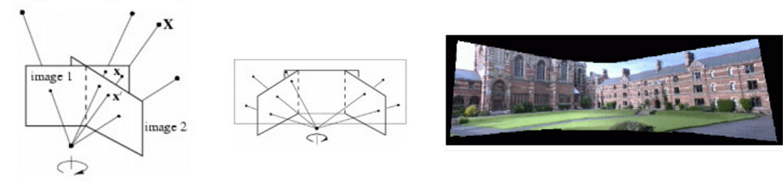
用 Blender 软件，获取相机只做旋转变换时的视图1和视图2，在已知相机标定矩阵和旋转矩阵的情况下，可计算出两个视图之间的单应性矩阵，从而完成拼接。

#include "opencv2/imgproc.hpp"
#include "opencv2/highgui.hpp"
#include "opencv2/calib3d.hpp"
 
using namespace cv;
 
int main()
{
    // 1) read image
    Mat img1 = imread("view1.jpg");
    Mat img2 = imread("view2.jpg");
    if (img1.empty() || img2.empty())
        return -1;
 
    // 2) camera pose from Blender at location 1
    Mat c1Mo = (Mat_<double>(4, 4) << 0.9659258723258972, 0.2588190734386444, 0.0, 1.5529145002365112,
                                      0.08852133899927139, -0.3303661346435547, -0.9396926164627075, -0.10281121730804443,
                                      -0.24321036040782928, 0.9076734185218811, -0.342020183801651, 6.130080699920654,
                                      0, 0, 0, 1);
    // camera pose from Blender at location 2
    Mat c2Mo = (Mat_<double>(4, 4) << 0.9659258723258972, -0.2588190734386444, 0.0, -1.5529145002365112,
                                      -0.08852133899927139, -0.3303661346435547, -0.9396926164627075, -0.10281121730804443,
                                      0.24321036040782928, 0.9076734185218811, -0.342020183801651, 6.130080699920654,
                                      0, 0, 0, 1);
    // 3) camera intrinsic parameters
    Mat cameraMatrix = (Mat_<double>(3, 3) << 700.0, 0.0, 320.0,
                                              0.0, 700.0, 240.0,
                                              0, 0, 1);
    // 4) extract rotation
    Mat R1 = c1Mo(Range(0, 3), Range(0, 3));
    Mat R2 = c2Mo(Range(0, 3), Range(0, 3));
 
    // 5) compute rotation displacement: c1Mo * oMc2
    Mat R_2to1 = R1 * R2.t();
 
    // 6) homography
    Mat H = cameraMatrix * R_2to1 * cameraMatrix.inv();
    H /= H.at<double>(2, 2);
 
    // 7) warp 
    Mat img_stitch;
    warpPerspective(img2, img_stitch, H, Size(img2.cols * 2, img2.rows));
 
    // 8) stitch
    Mat half = img_stitch(Rect(0, 0, img1.cols, img1.rows));
    img1.copyTo(half);
    imshow("Panorama stitching", img_stitch);
    waitKey();
}　　

输出结果如下：

视图1 视图2 拼接后的视图

参考资料：

OpenCV Tutorials / feature2d module / Basic concepts of the homography explained with code

Lecture 16: Planar Homographies, Robert Collins

Affine and Projective Transformations

posted on 2021-04-02 23:09 飞鸢逐浪阅读(1901) 评论(0) 编辑收藏举报

刷新页面返回顶部

登录后才能查看或发表评论，立即登录或者逛逛博客园首页

公告

昵称：飞鸢逐浪
园龄： 9年1个月
粉丝： 120
关注： 9

+加关注

2025年3月

日

一

二

三

四

五

六

合集

OpenCV 系列(15)

OpenCV 之平面单应性

1 投影变换

1.1 平面单应性

1.2 单应性矩阵

2 OpenCV 函数

2.1 投影变换矩阵

2.2 投影变换图像

3 代码示例

3.1 透视校正

3.2 图像拼接

参考资料：

公告

搜索

常用链接

我的标签

合集

随笔分类

随笔档案

阅读排行榜

评论排行榜

推荐排行榜

最新评论

OpenCV 之 平面单应性

1 投影变换

1.1 平面单应性

1.2 单应性矩阵

2 OpenCV 函数

2.1 投影变换矩阵

2.2 投影变换图像

3 代码示例

3.1 透视校正

3.2 图像拼接

参考资料：

公告

搜索

常用链接

我的标签

合集

随笔分类

随笔档案

阅读排行榜

评论排行榜

推荐排行榜

最新评论

OpenCV 之平面单应性