05机器学习实战之Logistic 回归scikit-learn实现

https://blog.csdn.net/zengxiantao1994/article/details/72787849似然函数

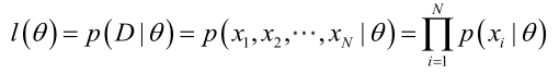
 原理：极大似然估计是建立在极大似然原理的基础上的一个统计方法，是概率论在统计学中的应用。极大似然估计提供了一种给定观察数据来评估模型参数的方法，即：“模型已定，参数未知”。通过若干次试验，观察其结果，利用试验结果得到某个参数值能够使样本出现的概率为最大，则称为极大似然估计。

    由于样本集中的样本都是独立同分布，可以只考虑一类样本集D，来估计参数向量θ。记已知的样本集为：

 似然函数（linkehood function）：联合概率密度函数称为相对于的θ的似然函数。

 https://blog.csdn.net/pql925/article/details/79021464对于似然函数的定义有些不正确，只看求导过程的推导

 

 

In [7]:

import numpy as np
import matplotlib.pyplot as plt

np.random.seed(666)
X = np.random.normal(0, 1, size=(200, 2))
y = np.array(X[:, 0] ** 2 + X[:, 1] < 1.5, dtype='int')

for _ in range(20):
    y[np.random.randint(200)] = 1  # 生成噪音数据
plt.scatter(X[y == 0, 0], X[y == 0, 1])
plt.scatter(X[y == 1, 0], X[y == 1, 1])
plt.show()

 

In [25]:

from sklearn.model_selection import train_test_split

X_train, X_test, y_train, y_test = train_test_split(X, y, random_state=666)

In [26]:

from sklearn.linear_model import LogisticRegression
from sklearn.preprocessing import PolynomialFeatures
from sklearn.pipeline import Pipeline

log_reg = LogisticRegression(solver='lbfgs')
log_reg.fit(X_train, y_train)

Out[26]:

LogisticRegression(C=1.0, class_weight=None, dual=False, fit_intercept=True,
          intercept_scaling=1, max_iter=100, multi_class='warn',
          n_jobs=None, penalty='l2', random_state=None, solver='lbfgs',
          tol=0.0001, verbose=0, warm_start=False)

In [27]:

log_reg.score(X_train, y_train)

Out[27]:

0.7933333333333333

In [28]:

log_reg.score(X_test, y_test)

Out[28]:

0.86

In [34]:

def plot_decision_boundary(model, axis):
    x0, x1 = np.meshgrid(
        np.linspace(axis[0], axis[1], int((axis[1] - axis[0]) * 100)),
        np.linspace(axis[2], axis[3], int((axis[3] - axis[2]) * 100))
    )
    X_new = np.c_[x0.ravel(), x1.ravel()]

    y_predict = model.predict(X_new)
    zz = y_predict.reshape(x0.shape)
    from matplotlib.colors import ListedColormap
    custom_cmap = ListedColormap(['#EF9A9A', '#FFF59D', '#90CAF9'])

    plt.contourf(x0, x1, zz, cmap=custom_cmap)

In [35]:

plot_decision_boundary(log_reg,axis=[-4,4,-4,4])
plt.scatter(X[y == 0, 0], X[y == 0, 1])
plt.scatter(X[y == 1, 0], X[y == 1, 1])
plt.show() 

 

 

多项式特征应用于逻辑回归

In [38]:

from sklearn.preprocessing import StandardScaler


def PolynomialLogisticRegression(degree):
    return Pipeline([
        ('Poly', PolynomialFeatures(degree=degree)),
        ('std_scaler', StandardScaler()),
        ('Logistic', LogisticRegression(solver='lbfgs'))
    ])


log_reg2 = PolynomialLogisticRegression(2)
log_reg2.fit(X_train, y_train)
log_reg2.score(X_train, y_train)

Out[38]:

0.9066666666666666

In [39]:

log_reg2.score(X_test, y_test)

Out[39]:

0.94

In [40]:

plot_decision_boundary(log_reg2, axis=[-4, 4, -4, 4])
plt.scatter(X[y == 0, 0], X[y == 0, 1])
plt.scatter(X[y == 1, 0], X[y == 1, 1])
plt.show()