膨胀卷积
膨胀卷积 Dilated Convolution
也叫空洞卷积 Atrous Convolution
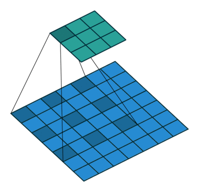
膨胀系数dilation rate \(r=1\)时就是普通卷积,上图中的膨胀系数\(r=2\)
为什么要引入膨胀卷积?
因为maxpooling进行池化操作后,一些细节和小目标会丢失,在之后的上采样中无法还原这些信息,造成小目标检测准确率降低
然而去掉池化层又会减小感受野
膨胀卷积的作用
- 增大感受野
- 保持输入特征的宽高
膨胀卷积的计算
For a convolution kernel with size \(k \times k\), the size of resulting dilated filter is \(k_d \times k_d\), where \(k_d = k + (k − 1) \cdot (r − 1)\)
比如下图的最左侧,\(r=2,k=3\)时,一个卷积核的总覆盖面积是\(5 \times 5\)
这里要注意实际的感受野其实就是\(k \times k\),因为插了0,实际参与到累加的pixel只有\(k \times k\)个
Since dilated convolution introduces zeros in the convolutional kernel, the actual pixels that participate in the computation from the \(k_d \times k_d\) region are just \(k \times k\), with a gap of \(r − 1\) between them.
膨胀卷积的问题
栅格效应Gridding Effect
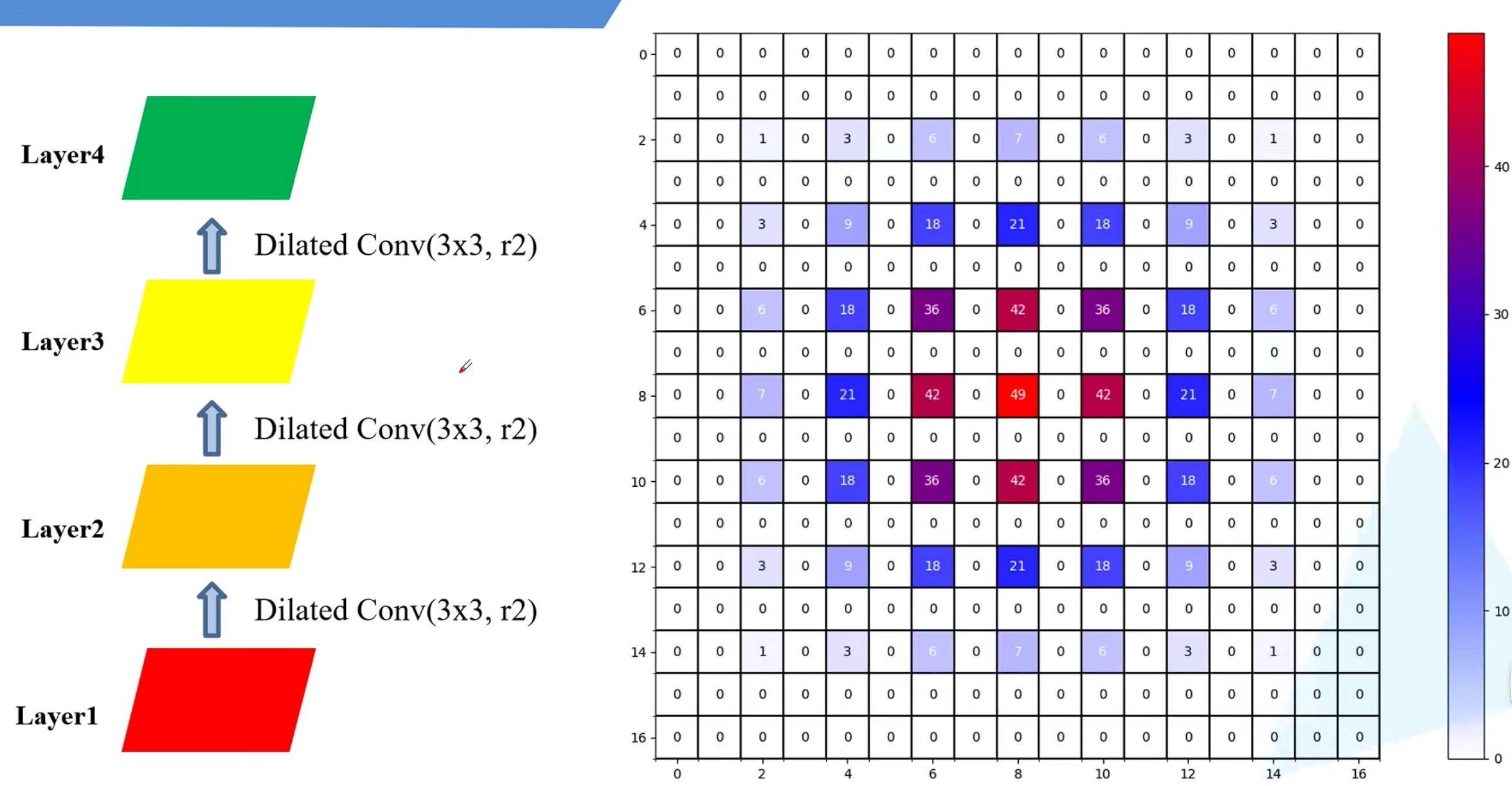
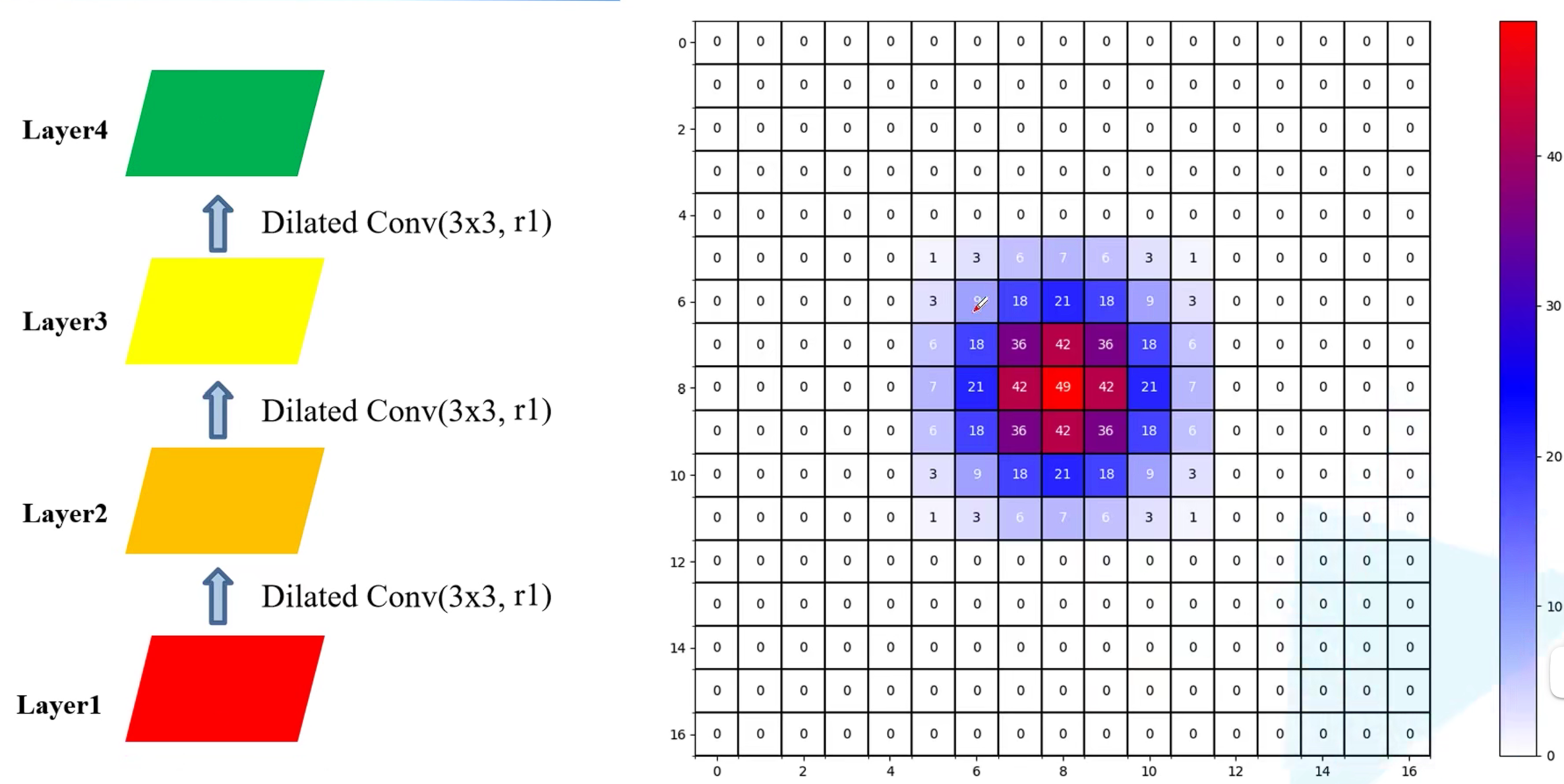
用上图解释一下,如果经过三次膨胀系数\(r=2\),kernel size=\(3\times 3\)的膨胀卷积
第二层的一个pixel用到了第一层的9个pixel,如最左图所示,接着第三层的一个pixel就用到了第二层的9个pixel,也就相当于第一层的25个pixel,如中间图所示
颜色代表通过累加,第一层的各个pixel被当前层利用到的次数,次数越高颜色越深
最后就是下图效果
从上图可以看出Dilated Convolution的kernel并不连续,也就是并不是所有的像素都用来计算了,因此这里将信息看作checker-board的方式将会损失信息的连续性
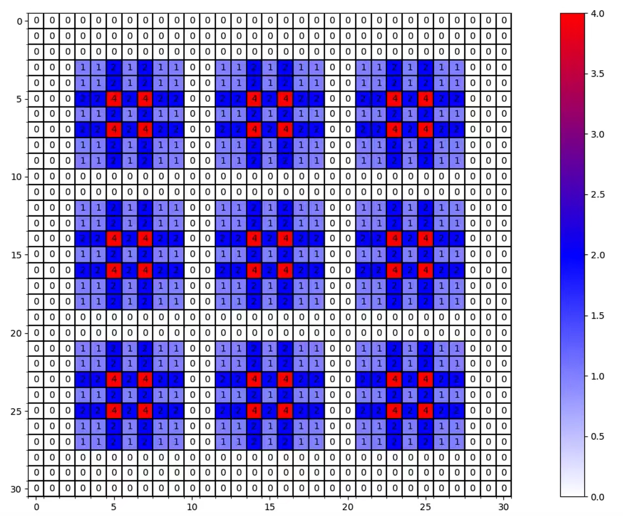
而如果第一次采用普通卷积的话就不会丢失底层信息,接着采用不同的膨胀系数,感受野跟上一种方法是一样大的却能利用到更多的信息
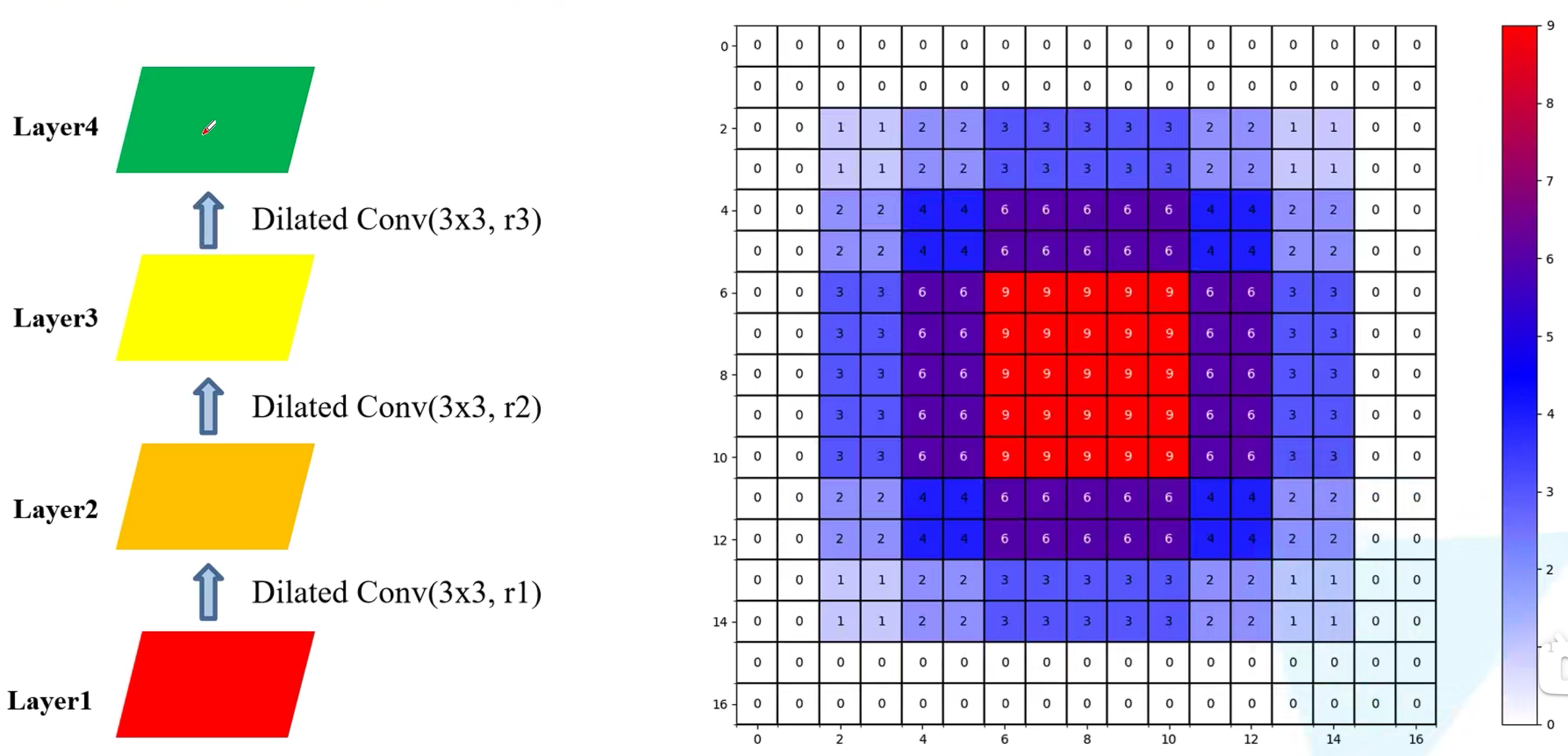
再与普通卷积对比一下,普通卷积虽然利用了连续的区域,但相比之下感受野就小了很多
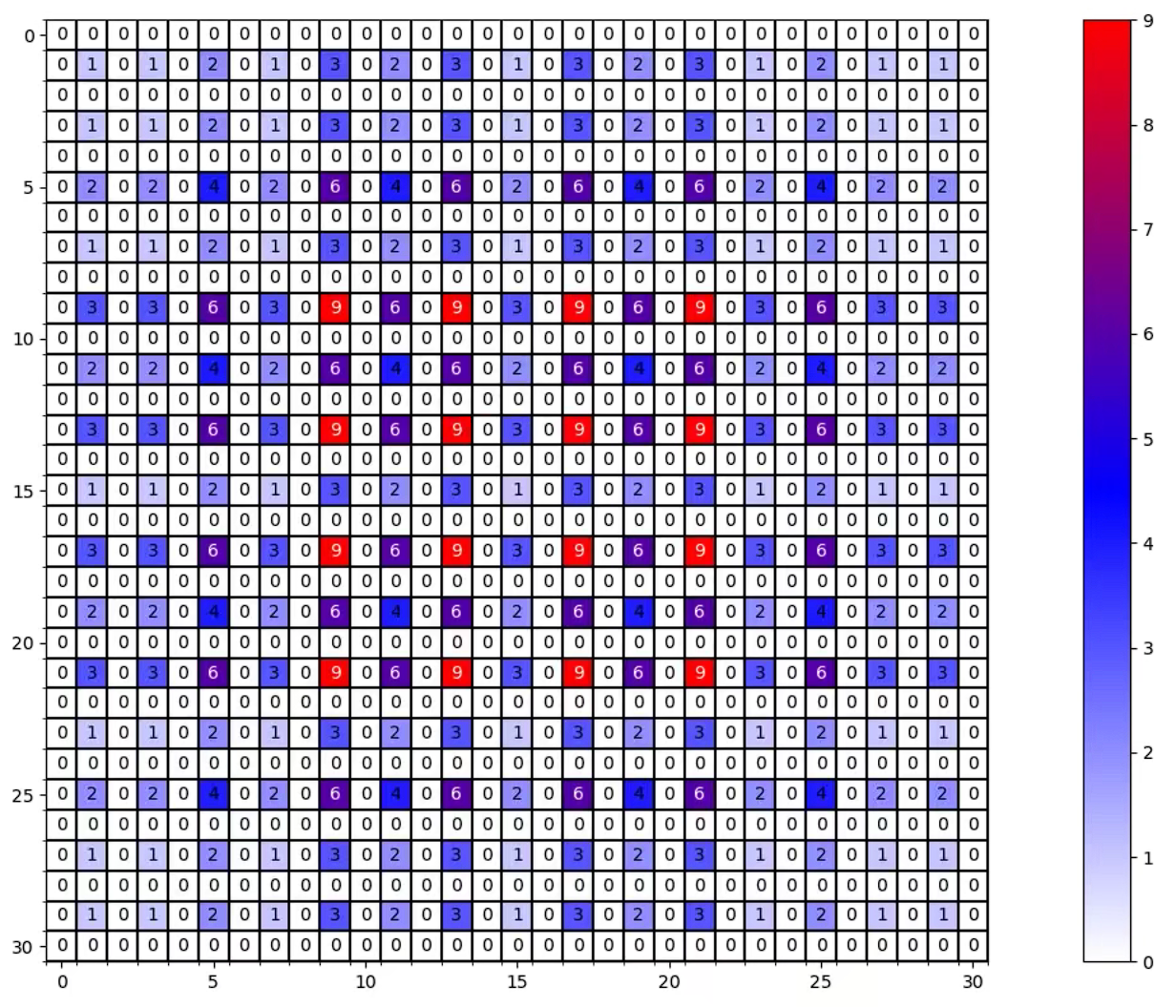
Hybrid Dilated Convolution(HDC)
非零元素最大距离
当使用到多个膨胀卷积时,需要设计各卷积核的膨胀系数使其刚好能覆盖底层特征层
The goal of HDC is to let the final size of the RF of a series of convolutional operations fully covers a square region without any holes or missing edges.
论文中提到了maximum distance between two nonzero values,通过这个来限制膨胀系数的大小

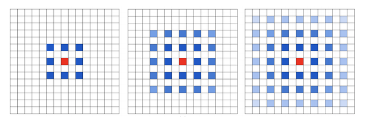
下图分别为\(r=\)[1,2,5]和[1,2,9]的情况

锯齿结构
dilated rate设计成了锯齿状结构,例如[1, 2, 5, 1, 2, 5]这样的循环结构
公约数不能大于1
叠加的膨胀卷积的膨胀率dilated rate不能有大于1的公约数(比如[2, 4, 8]),不然会产生栅格效应
画图代码
import numpy as np
import matplotlib.pyplot as plt
from matplotlib.colors import LinearSegmentedColormap


def dilated_conv_one_pixel(center: (int, int),
                           feature_map: np.ndarray,
                           k: int = 3,
                           r: int = 1,
                           v: int = 1):
    """
    膨胀卷积核中心在指定坐标center处时,统计哪些像素被利用到,
    并在利用到的像素位置处加上增量v
    Args:
        center: 膨胀卷积核中心的坐标
        feature_map: 记录每个像素使用次数的特征图
        k: 膨胀卷积核的kernel大小
        r: 膨胀卷积的dilation rate
        v: 使用次数增量
    """
    assert divmod(3, 2)[1] == 1

    # left-top: (x, y)
    left_top = (center[0] - ((k - 1) // 2) * r, center[1] - ((k - 1) // 2) * r)
    for i in range(k):
        for j in range(k):
            feature_map[left_top[1] + i * r][left_top[0] + j * r] += v


def dilated_conv_all_map(dilated_map: np.ndarray,
                         k: int = 3,
                         r: int = 1):
    """
    根据输出特征矩阵中哪些像素被使用以及使用次数,
    配合膨胀卷积k和r计算输入特征矩阵哪些像素被使用以及使用次数
    Args:
        dilated_map: 记录输出特征矩阵中每个像素被使用次数的特征图
        k: 膨胀卷积核的kernel大小
        r: 膨胀卷积的dilation rate
    """
    new_map = np.zeros_like(dilated_map)
    for i in range(dilated_map.shape[0]):
        for j in range(dilated_map.shape[1]):
            if dilated_map[i][j] > 0:
                dilated_conv_one_pixel((j, i), new_map, k=k, r=r, v=dilated_map[i][j])

    return new_map


def plot_map(matrix: np.ndarray):
    plt.figure()

    c_list = ['white', 'blue', 'red']
    new_cmp = LinearSegmentedColormap.from_list('chaos', c_list)
    plt.imshow(matrix, cmap=new_cmp)

    ax = plt.gca()
    ax.set_xticks(np.arange(-0.5, matrix.shape[1], 1), minor=True)
    ax.set_yticks(np.arange(-0.5, matrix.shape[0], 1), minor=True)

    # 显示color bar
    plt.colorbar()

    # 在图中标注数量
    thresh = 5
    for x in range(matrix.shape[1]):
        for y in range(matrix.shape[0]):
            # 注意这里的matrix[y, x]不是matrix[x, y]
            info = int(matrix[y, x])
            ax.text(x, y, info,
                    verticalalignment='center',
                    horizontalalignment='center',
                    color="white" if info > thresh else "black")
    ax.grid(which='minor', color='black', linestyle='-', linewidth=1.5)
    plt.show()
    plt.close()

def main():
    # bottom to top
    dilated_rates = [1, 2, 3]
    # init feature map
    size = 31
    m = np.zeros(shape=(size, size), dtype=np.int32)
    center = size // 2
    m[center][center] = 1
    # print(m)
    # plot_map(m)

    for index, dilated_r in enumerate(dilated_rates[::-1]):
        new_map = dilated_conv_all_map(m, r=dilated_r)
        m = new_map
    print(m)
    plot_map(m)

if __name__ == '__main__':
    main()