
人工智能
机器学习
a^2+b^2 = c^2
c= np.sqrt(a**2+b**2)
理性主义
经验主义
通过大量的数据,让计算机系统掌握数据之间的内在联系,进而对未知的结果做出预测,这样的系统谓之机器学习过程。
机器学习的过程就是发现数据之间内在联系的过程
第一步:数据采集、挖掘和清洗 --买菜
第二步:数据预处理(让算法简单一点)--洗菜和切菜
第三步:模型选择 -- 制定菜谱
第四步:模型训练 -- 烹饪
第五步:模型测试 -- 试吃
第六步:使用模型 -- 上桌
一、数据预处理
1、均值移除(标准化):各列特征的 平均值为0,标准差为1
*2
+----+
输入数据->|模型|<-输出数据
+----+
1 2
2 4
3 6
...
100 *2 200 ==200 OK
测试
1000 *2 2000 ->信任,业务
使用
样本矩阵 特征1 特征2 特征3 ... 特征n -->标签向量
样本1 x x x ... x y
样本2 x x x ... x y
样本3 x x x ... x y
... ...
样本n x x x ... x y
一行一样本,一列一特征
年龄 学历 学校 工作经历 --> 薪资
25 专科 普通 没有 3000
28 本科 985 2 6000
35 博士 211 5 10000
...
27 硕士 普通 3 ?
使样本矩阵中的各列的平均值为0,标准差为1,即将每个特征的基准位置和分散度加以统一,在数量级上尽可能接近,对模型的预测结果做出均等的贡献
体征i
a
b
c
m = (a+b+c)/3
a' = a-m
b' = b-m
c' = c-m
m' = (a'+b'+c')/3
= (a-m + b-m + c-m)/3
= (a+b+c)/3 - m
= 0
s' = sqrt((a'^2+b'^2+c'^2)/3)
a''= a'/s'
b''= b/s'
c''= c'/s'
s''=sqrt((a''^2+b''^2+c''^2)/3)
=sqrt((a'^2/s'^ + b'^2/s'^ + c'^2/s'^)/3)
=sqrt((a'^2 + b'^2 + c'^2)+/(3s'^2))
=sqrt(3s'^2/3s'^2)
=1
总结:让每列的值减去这一列的平均值然后在除以这一列数据的标准差,获取新的列
安装:pip instanll scikit-learn
import sklearn.preprocessing as sp
sp.scale(原始样本矩阵)->均值移除样本矩阵
import numpy as np
import sklearn.preprocessing as sp

raw_samples = np.array([
    [3, -1.5, 2, -5.4],
    [0, 4, -0.3, 2.1],
    [1, 3.3, -1.9, -4.3]
])
print(raw_samples)
# axis=0代表垂直方向
# 平均值
mean = raw_samples.mean(axis=0)
print(mean)  # [ 1.33333333  1.93333333 -0.06666667 -2.53333333]
# 标准差
std = raw_samples.std(axis=0)
print(std)  # [ 1.24721913  2.44449495  1.60069429  3.30689515]
# 将每列的元素都减去每列的平均值
std_samples = raw_samples.copy()
std_samples = (std_samples - mean)/std
print(std_samples)
# 平均值变为0
mean = std_samples.mean(axis=0)
print(mean)  # [  5.55111512e-17  -1.11022302e-16  -7.40148683e-17  -7.40148683e-17]
# 标准差变为1
std = std_samples.std(axis=0)
print(std)  # [ 1.  1.  1.  1.]
#  使用sklearn
std_samples = sp.scale(raw_samples)
print(std_samples.mean(axis=0))  # [  5.55111512e-17  -1.11022302e-16  -7.40148683e-17  -7.40148683e-17]
print(std_samples.std(axis=0))  # [ 1.  1.  1.  1.]
2、范围缩放
语文 数学 英语(每课的总分不一样)
张三 90 10(100)5(100)
李四 80 8(80) 2(40)
王五 100 5(5) 1(20)
将样本矩阵中的每一列通过线性变换,使各列的最大值和最小值为某个给定的值,即分布在相同的范围中
线性变换:kx + b = y
每列的最小值:k*col_min + 1b = min
每列的最大值:K*col_max + 1b = max
/col_min 1\ * /k\ = /min\
\col_max 1/ \b/ \max/
---------- ---- -----
a x b
= numpy.linalg.solve(a,b)
mms = sp.MinMaxScaler(feature_range=(min,max))
mms.fit_transform(原始样本矩阵)->范围缩放样本矩阵
import numpy as np
import sklearn.preprocessing as sp


raw_samples = np.array([
    [3, -1.5, 2, -5.4],
    [0, 4, -0.3, 2.1],
    [1, 3.3, -1.9, -4.3]
])
print(raw_samples)
mms_samples = raw_samples.copy()
for col in mms_samples.T:
    col_min = col.min()
    col_max = col.max()
    a = np.array([[col_min, 1],[col_max,1]])
    # 让每列的数据都砸0和1之间
    b = np.array([0,1])
    x = np.linalg.solve(a, b)
    col *= x[0]
    col += x[1]
print(mms_samples)
mms = sp.MinMaxScaler(feature_range=(0,1))
mms_samples = mms.fit_transform(raw_samples)
print(mms_samples)
3、归一化
C/C++ Java Python PHP
2016 30 40 10 5 /85
2017 30 35 40 1 /106
2018 20 30 50 0 /100
将样本矩阵中的每一列的特征值除以一行中总的样本数,使得每行样本的总数为1
sp.normalize(原始样本矩阵,norm=‘l1’)-->经过归一化样本矩阵
L1范数: 向量中各元素绝对值之和
L2范数:向量中各元素的平方之和
import numpy as np
import sklearn.preprocessing as sp
raw_samples = np.array([
    [3, -1.5, 2, -5.4],
    [0, 4, -0.3, 2.1],
    [1, 3.3, -1.9, -4.3]
])
print(raw_samples)
nor_samples = raw_samples.copy()
for row in nor_samples:
    # 求每行样本的总数
    row_absum = abs(row).sum()
    row /= row_absum
print(nor_samples)
# 按行取值
print(abs(nor_samples).sum(axis=1))  # [ 1.  1.  1.]
nor_samples = sp.normalize(raw_samples,norm='l1')
print(nor_samples)
print(abs(nor_samples).sum(axis=1))
nor_samples = sp.normalize(raw_samples,norm='l2')
print(nor_samples)
print(abs(nor_samples).sum(axis=1))
4、二值化
根据业务的需求,设定一个阈值,样本矩阵中大于阈值的元素被置为1,小于等于阈值的元素被置为0,整个样本矩阵被处理为只有0和1组成样本空间
bin = sp.Binarizer(threshold=阈值)
bin.transform(原始样本矩阵)-->二值化样本矩阵
import numpy as np
import sklearn.preprocessing as sp
raw_samples = np.array([
    [3, -1.5, 2, -5.4],
    [0, 4, -0.3, 2.1],
    [1, 3.3, -1.9, -4.3]
])
print(raw_samples)
bin_samples = raw_samples.copy()
bin_samples[bin_samples <= 1.4] = 0
bin_samples[bin_samples > 1.4] = 1
print(bin_samples)
bin = sp.Binarizer(threshold=1.4)
bin_samples = bin.transform(raw_samples)
print(bin_samples)
5、独热编码
1 3 2
7 5 4
1 8 6
7 3 9
1:10 3:100 2:1000
7:01 5:010 4:0100
8:001 6:0010
9:0001
将每一列的特征值使用1个1和多个0组合表示,0和1的总个数由每列特征值的数值个数来决定
ohe = sp.OneHotEncoder(sparse=是否压缩, dtype=类型)
ohe.fit_transform(原始样本矩阵)-->独热编码样本逆矩阵
import numpy as np
import sklearn.preprocessing as sp
raw_samples = np.array([
    [1, 3, 2],
    [7, 5, 4],
    [1, 8, 6],
    [7, 3, 9]
])
# 编码表
code_tables = []
for col in raw_samples.T:
    code_table = {}
    for val in col:
        code_table[val] = None
    code_tables .append(code_table)
print(code_tables)
for code_table in code_tables:
    # 求出字典键的个数
    size = len(code_table)
    for one, key in enumerate(sorted(code_table.keys())):
        code_table[key] = np.zeros(shape=size, dtype=int)
        code_table[key][one] = 1
print(code_tables)
ohe_samples = []
for raw_sample in raw_samples:
    ohe_sample = np.array([], dtype=int)
    for i, key in enumerate(raw_sample):
        # 水平组合
        ohe_sample = np.hstack((ohe_sample, code_tables[i][key]))
    ohe_samples.append(ohe_sample)
ohe_samples = np.array(ohe_samples)
print(ohe_samples)
# 创建独热编码器
ohe = sp.OneHotEncoder(sparse=False, dtype=int)
ohe_samples = ohe.fit_transform(raw_samples)
print(ohe_samples)
'''
sparse=False的结果
[[1 0 1 0 0 1 0 0 0]
 [0 1 0 1 0 0 1 0 0]
 [1 0 0 0 1 0 0 1 0]
 [0 1 1 0 0 0 0 0 1]]
 sparse=True的结果,稀疏矩阵0多1少
  (0, 5)    1 # 表示第0行第5列为1
  (0, 2)    1
  (0, 0)    1
  (1, 6)    1
  (1, 3)    1
  (1, 1)    1
  (2, 7)    1
  (2, 4)    1
  (2, 0)    1
  (3, 8)    1
  (3, 2)    1
  (3, 1)    1
'''
new_sample = np.array([[1, 5, 6]])
# 此时编码字典已经存在ohe中,无需调用fit_transform,增加的新样本能出现行的特征值
ohe_sample = ohe.transform(new_sample)
print(ohe_sample)
6、标签编码
年龄 学历 学校 工作经历 --> 薪资
25 专科 普通 没有 low
28 本科 985 2 med
35 博士 211 5 high
...
27 硕士 普通 3 ?
将字符串形式的特征值编码成数字,便于数学运算。
low med high
排序
high low med
0 1 2
编码:1 2 0
标签编码器:lbe = sp.LabelEncoder()
lbe.fit_transform(原始样本矩阵列) -->标签编码列,构建字典
lbe.transform(原始样本矩阵列) --> 标签编码列,使用字典
lbe.inverse_transform(标签编码列) --> 原始样本列, 使用字典
import numpy as np
import sklearn.preprocessing as sp
raw_samples = np.array([
    'audi', 'ford', 'audi', 'toyota','ford', 'bmw', 'toyota', 'ford'
])
print(raw_samples)
lbe = sp.LabelEncoder()
lbe_sample = lbe.fit_transform(raw_samples)
print(lbe_sample)
new_sample = np.array(['bmw', 'audi', 'toyota'])
lbe_sample = lbe.transform(new_sample)
print(lbe_sample)
# 求逆
raw_samples = lbe.inverse_transform(lbe_sample)
print(raw_samples)
二、机器学习基本类型
1、有监督学习:用已知的输入和输出训练学习模型(f(x)),直到模型给出的预测输出与已知的实际输出之间的误差小到可以接受程度为止
x1 -> y1
x2 -> y2
x3 -> y3
...
y=f(x)
x1 -> y1'
x2 -> y2'
x3 -> y3'
1、回归问题:输出数据是无限可能的连续值
2、分类问题:输出数据是有限的几个离散值
2、无监督学习:在输出数据未知的前提下,利用模型本身发现输入数据的内部特征,将其划分为不同的族群
聚类问题
3、半监督学习:利用相对较小的已知集训练模型,使其获得基本的预测能力,当模型遇到未知输出的新数据时,可以根据其与已知集的相似性们预测其输出
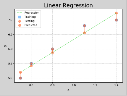
三、线性回归
x --> y
0.5 5.0
0.6 5.5
0.8 6.0
1.1 6.8
1.4 7.0
预测函数:yi = w0 + w1x
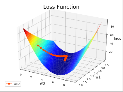
SUM([y - (w0 + w1x)]^2)
loss = -----------------------------------
2
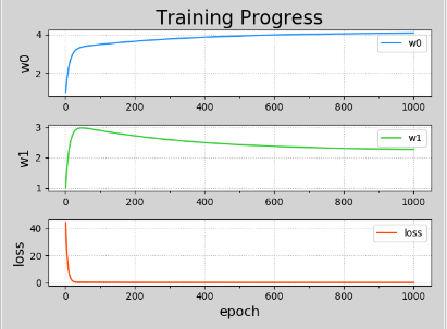
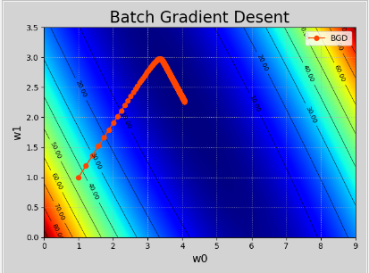
目标:寻找最理想的w0和w1,使loss(损失值)尽可能的小。

dloss
loss对w0的偏导 : ---------- = -SUM(y - (w0 + w1x))
dwo
dloss
loss对w1的偏导: ---------- = -SUM([y - (w0 + w1x)]x)
dw1
dloss
w0 = w0 - n(学习率) * ----------
dw0
dloss
w1 = w1 - n(学习率)* --------
dw1
# 自己写一个类实现上面求解斜率和截距的过程
import numpy as np
import matplotlib.pyplot as plt
%matplotlib inline
class Linera_model(object):
    def __init__(self):
        # 初始化斜率
        self.w = np.random.randn(1)[0]
        # 初始化截距
        self.b = np.random.randn(1)[0]
        print("-----------初始值",self.w, self.b)
    # 创建函数方程y = wx + b
    def model(self, x):
        return self.w * x + self.b
    def loss(self, x, y):
        cost = ((y - self.model(x))**2)/2
        # 对w求偏导(就是把b看做常量的求导)
        g_w = (y - self.model(x)) * (-x)
        # 对b求偏导
        g_b = (y - self.model(x)) * (-1)
        return g_w, g_b
    # 梯度下降
    def gradient_descend(self, g_w, g_b, step=0.01):
        # 更新斜率和截距, step相当于学习率
        self.w = self.w - g_w * step
        self.b = self.b - g_b * step
        print("-----------",self.w, self.b)
    def fit(self, X, y):
        # 初始化上一次的斜率和截距
        last_w = self.w + 1
        last_b = self.b + 1
        # 设置精度和循环最大次数
        precision = 0.00001
        max_count = 3000
        count = 0
        while True:
            if (np.abs(last_w - self.w) < precision) and (np.abs(last_b - self.b) < precision):
                break
            if count > max_count:
                break
            # 更新斜率和截距
            g_w = 0
            g_b = 0
            size = X.shape[0]
            for xi, yi in zip(X, y):
                g_w += self.loss(xi, yi)[0] / size
                g_b += self.loss(xi, yi)[1] / size
            self.gradient_descend(g_w, g_b)
            count += 1
    @property
    def coef_(self):
        return self.w
    @property
    def intercept_(self):
        return self.b
lm = Linera_model()
X = np.linspace(2.5, 12, 25)
w = np.random.randint(2, 10, size=1)[0]
b = np.random.randint(-5, 5, size=1)[0]
y = X * w + b + np.random.randn(25)*2
plt.scatter(X, y)
lm.fit(X, y)
print(lm.coef_, lm.intercept_)
import numpy as np
import matplotlib.pyplot as mp
from mpl_toolkits.mplot3d import axes3d
train_x = np.array([0.5,0.6,0.8,1.1,1.4])
train_y = np.array([5.0,5.5,6.0,6.8,7.0])
# 迭代次数
n_epoches = 1000
# 学习率
lrate = 0.01
epoches, losses = [],[]
w0, w1 = [1],[1]
for epoch in range(1,n_epoches+1):
    epoches.append(epoch)
    losses.append(((train_y - (w0[-1] + w1[-1]*train_x))**2).sum()/2)
    print('{:4} w0={:.8f}, w1={:8}, loss={:.8f}'.format(epoches[-1],w0[-1],w1[-1],losses[-1]))
    d0 = -(train_y - (w0[-1] + w1[-1]*train_x)).sum()
    d1 = -((train_y - (w0[-1] + w1[-1]*train_x))*train_x).sum()
    w0.append(w0[-1] - lrate *d0)
    w1.append(w1[-1] - lrate *d1)
w0 = np.array(w0[:-1])
w1 = np.array(w1[:-1])
# 排序
sorted_indices = train_x.argsort()
test_x = train_x[sorted_indices]
test_y = train_y[sorted_indices]
pred_test_y = w0[-1] + w1[-1] *test_x
# 画曲面图
grid_w0, grid_w1 = np.meshgrid(np.linspace(0, 9, 500),np.linspace(0, 3.5, 500))
flat_w0, flat_w1 = grid_w0.ravel(), grid_w1.ravel()
# 损失值
flat_loss = ((flat_w0 + np.outer(train_x, flat_w1) -train_y.reshape(-1,1))**2).sum(axis=0)/2
# 网格化
grid_loss = flat_loss.reshape(grid_w0.shape)
mp.figure('Linear Regression', facecolor='lightgray')
mp.title('Linear Regression', fontsize=20)
mp.xlabel('x', fontsize=14)
mp.ylabel('y', fontsize=14)
mp.tick_params(labelsize=10)
mp.grid(linestyle=':')
# marker='s'表示方点
mp.scatter(train_x, train_y, marker='s',c='dodgerblue',alpha=0.5,s=80,label='Training')
mp.scatter(test_x, test_y, marker='D',c='orangered',alpha=0.5,s=60,label='Testing')
mp.scatter(test_x, pred_test_y,c='orangered',alpha=0.5,s=80,label='Predicted')
# 误差
for x, y, pred_y in zip(test_x, test_y, pred_test_y):
    mp.plot([x, x], [y, pred_y], c='orangered', alpha=0.5,linewidth=1)
mp.plot(test_x,pred_test_y,'--', c='limegreen', label='Regression', linewidth=1)
mp.legend()
mp.figure('Training Progress', facecolor='lightgray')
mp.subplot(311)
mp.title("Training Progress", fontsize=20)
mp.ylabel('w0', fontsize=14)
mp.gca().xaxis.set_minor_locator(mp.MultipleLocator(100))
mp.tick_params(labelsize=10)
mp.grid(linestyle=':')
mp.plot(epoches, w0, c='dodgerblue', label='w0')
mp.legend()
mp.subplot(312)
mp.ylabel('w1', fontsize=14)
mp.gca().xaxis.set_minor_locator(mp.MultipleLocator(100))
mp.tick_params(labelsize=10)
mp.grid(linestyle=':')
mp.plot(epoches, w1, c='limegreen', label='w1')
mp.legend()
mp.subplot(313)
mp.xlabel('epoch',fontsize=14)
mp.ylabel('loss', fontsize=14)
mp.gca().xaxis.set_minor_locator(mp.MultipleLocator(100))
mp.tick_params(labelsize=10)
mp.grid(linestyle=':')
mp.plot(epoches, losses, c='orangered', label='loss')
mp.legend()
mp.tight_layout()
mp.figure('Loss Function')
ax = mp.gca(projection='3d')
mp.title('Loss Function', fontsize=20)
ax.set_xlabel('w0', fontsize=14)
ax.set_ylabel('w1', fontsize=14)
ax.set_zlabel('loss', fontsize=14)
mp.tick_params(labelsize=10)
ax.plot_surface(grid_w0, grid_w1, grid_loss, rstride=10, cstride=10, cmap='jet')
ax.plot(w0, w1, losses, 'o-', c='orangered', label='GBD')
mp.legend(loc='lower left')
mp.figure('Batch Gradient Desent', facecolor='lightgray')
mp.title('Batch Gradient Desent', fontsize=20)
mp.xlabel('w0', fontsize=14)
mp.ylabel('w1', fontsize=14)
mp.tick_params(labelsize=10)
mp.grid(linestyle=':')
mp.contourf(grid_w0, grid_w1, grid_loss, 1000, cmap='jet')
cntr = mp.contour(grid_w0, grid_w1, grid_loss, 10, colors='black', linewidths=0.5)
mp.clabel(cntr, inline_space=0.1, fmt='%.2f', fontsize=8)
mp.plot(w0, w1, 'o-', c='orangered', label='BGD')
mp.legend()
mp.show()
import sklearn.linear_model as lm
model = lm.LinearRegression() # 创建模型
model.fit(训练输入,训练输出) # 训练模型
预测输出 = model.predict(预测输入) # 预测输出
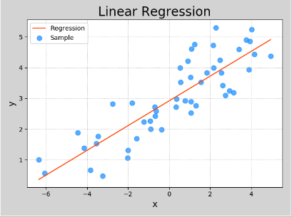
import numpy as np
import sklearn.linear_model as lm
import sklearn.metrics as sm
import matplotlib.pyplot as mp
import pickle


x , y = [], []
with open('../data/single.txt', 'r') as f:
    for line in f.readlines():
        data = [float(substr) for substr in line.split(',')]
        x.append(data[:-1])
        y.append(data[-1])
x = np.array(x)
y = np.array(y)
print(x)
print(y)
# 创建模型
model = lm.LinearRegression()
# 训练模型
model.fit(x, y)
# 预测模型
pred_y = model.predict(x)
print(sm.mean_absolute_error(y, pred_y))
print(sm.mean_squared_error(y, pred_y))
print(sm.median_absolute_error(y, pred_y))
print(sm.r2_score(y, pred_y))  # 越接近1越好
# 保存模型
with open('../data/linear.pkl','wb') as f:
    pickle.dump(model, f)
# 加载模型
with open('../data/linear.pkl', 'rb') as f:
    model = pickle.load(f)
pred_y = model.predict(x)
print(sm.mean_absolute_error(y, pred_y))
print(sm.mean_squared_error(y, pred_y))
print(sm.median_absolute_error(y, pred_y))
print(sm.r2_score(y, pred_y))  # 越接近1越好
mp.figure('Linear Regression', facecolor='lightgray')
mp.title('Linear Regression', fontsize=20)
mp.xlabel('x', fontsize=14)
mp.ylabel('y', fontsize=14)
mp.tick_params(labelsize=10)
mp.grid(linestyle=':')
mp.scatter(x, y, c='dodgerblue', alpha=0.75, s=60, label='Sample')
sorted_indices = x.T[0].argsort()
mp.plot(x[sorted_indices], pred_y[sorted_indices], c='orangered', label='Regression')
mp.legend()
mp.show()
模型保存:
import pickle
with open(模型文件路径) as f:
pickle.dump(model, f) # 将学习模型保存到文件
加载模型
with open(模型文件路径) as f:
model = pickle.load(f) # 从文件中载入学习模型
四、岭回归
loss = J(w0, w1) + 正则强度(惩罚力度) * 正则项(x,y,w0,w1)
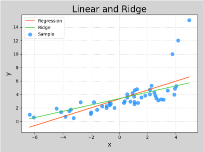
领回归就是在线性回归的基础上增加了正则项,有意破坏模型对训练数据集的拟合效果,客观上降低了少数异常样本对模型的牵制作用,
使得模型对大多数正常样本表现出更好的拟合效果
model = lm.Ridge(正则强度,fit_intercept=True,max_iter=最大迭代次数)
model.fit(训练输入,训练输出)
预测输入 = model.predict(预测输入)
import numpy as np
import sklearn.linear_model as lm
import sklearn.metrics as sm
import matplotlib.pyplot as mp
x , y = [], []
with open('../data/abnormal.txt', 'r') as f:
    for line in f.readlines():
        data = [float(substr) for substr in line.split(',')]
        x.append(data[:-1])
        y.append(data[-1])
x = np.array(x)
y = np.array(y)
print(x)
print(y)
# 创建模型
model_ln = lm.LinearRegression()
# 训练模型
model_ln.fit(x, y)
# 预测模型
pred_y_ln = model_ln.predict(x)
print(sm.mean_absolute_error(y, pred_y_ln))
print(sm.mean_squared_error(y, pred_y_ln))
print(sm.median_absolute_error(y, pred_y_ln))
print(sm.r2_score(y, pred_y_ln))  # 越接近1越好
# fit_intercept=True时,截距(w0),斜率(w1)都会受到影响。为False时,只影响w1
model_rd = lm.Ridge(150, fit_intercept=True, max_iter=10000)
model_rd.fit(x, y)
pred_y_rd = model_rd.predict(x)
print(sm.mean_absolute_error(y, pred_y_rd))
print(sm.mean_squared_error(y, pred_y_rd))
print(sm.median_absolute_error(y, pred_y_rd))
print(sm.r2_score(y, pred_y_rd))
mp.figure('Linear and Ridge', facecolor='lightgray')
mp.title('Linear and Ridge', fontsize=20)
mp.xlabel('x', fontsize=14)
mp.ylabel('y', fontsize=14)
mp.tick_params(labelsize=10)
mp.grid(linestyle=':')
mp.scatter(x, y, c='dodgerblue', alpha=0.75, s=60, label='Sample')
sorted_indices = x.T[0].argsort()
mp.plot(x[sorted_indices], pred_y_ln[sorted_indices], c='orangered', label='Regression')
mp.plot(x[sorted_indices], pred_y_rd[sorted_indices], c='limegreen', label='Ridge')
mp.legend()
mp.show()
五、多项式回归
y = w0 + w1x + w2x^2 + w3x^3 + ... + wnx^n
x1 = x
x2 = x^2
x3 = x^3
....
xn = x^n
y = w0 + w1x + w2x2 + w3x3 + ... + wnxn
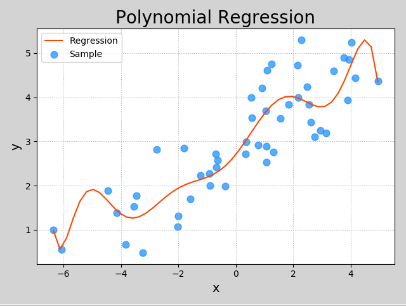
多项式特征扩展:增加高次项作为扩展特征值;沿用线性回归对增补了扩展值后的样本矩阵进行回归
import sklearn.pipline as pl
import sklearn.preprocessing as sp
....
sp.PolynomialFeatures(n)->多项式特征扩展器
lm.LinearRegression()->线性回归
pl.make_pipline(多项式特征扩展器,线性回归器)->管线
管线.fit()
管线.predict()->预测输出
x -> 多项式特征扩展器 ->x1,x2,x3,...,xn ->线性回归器 ->w0 w1 ...wn
\______________________________________________/
|
管线(流水线)
欠拟合:模型中的参数并不能以最佳损失值的形式来反映输入和输出之间的关系。因此,无论是用训练集输入还是测试集输入,
由模型给出的预测输出都不能以较小的误差接近实际的输出
过拟合:模型中的参数过分依赖或者倾向于训练数据,反而缺乏一般性,即导致泛化程度的缺失。因此当使用训练集输入时,模型通常可以给出
较高精度的预测输出,而使用测试集输入,模型的表现却非常差
import numpy as np
import sklearn.linear_model as lm
import sklearn.pipeline as pl
import sklearn.preprocessing as sp
import sklearn.metrics as sm
import matplotlib.pyplot as mp
train_x , train_y = [], []
with open('../data/single.txt', 'r') as f:
    for line in f.readlines():
        data = [float(substr) for substr in line.split(',')]
        train_x.append(data[:-1])
        train_y.append(data[-1])
train_x = np.array(train_x)
train_y = np.array(train_y)
print(train_x)
print(train_y)
# 多项式扩展器, 线性回归
model =pl.make_pipeline(sp.PolynomialFeatures(10), lm.LinearRegression())
model.fit(train_x, train_y)
pred_train_y = model.predict(train_x)
# 列向量
test_x = np.linspace(train_x.min(), train_x.max(),50)[:,np.newaxis]
pred_test_y = model.predict(test_x)
print(sm.r2_score(train_y, pred_test_y))
mp.figure('Polynomial Regression', facecolor='lightgray')
mp.title('Polynomial Regression', fontsize=20)
mp.xlabel('x', fontsize=14)
mp.ylabel('y', fontsize=14)
mp.tick_params(labelsize=10)
mp.grid(linestyle=':')
mp.scatter(train_x, train_y, c='dodgerblue', alpha=0.75, s=60, label='Sample')
mp.plot(test_x, pred_test_y, c='orangered', label='Regression')
mp.legend()
mp.show()
分别使用线性回归、岭回归、多项式回归对波士顿房价进行预测


 1 import pandas as pd
 2 import matplotlib.pyplot as plt
 3 from sklearn import datasets
 4 from sklearn.model_selection import train_test_split
 5 from sklearn import linear_model as lm
 6 from sklearn import pipeline
 7 from sklearn.metrics import r2_score
 8 from sklearn.preprocessing import MinMaxScaler, PolynomialFeatures
 9
10
11 # 1、加载数据
12 boston = datasets.load_boston()
13 data = pd.DataFrame(boston.data, columns=boston.feature_names)
14 data["TARGET"] = boston.target
15
16 # 2、特征分析
17 print(data.describe())
18 # 对某些字段进行简单的数据分析,
19 print(data.pivot_table(index="CHAS", values=["TARGET"]))
20 # 如果想使用这组数据训练线性模型,则要先检验特征与输出之间的关系是否存在线性关系
21 data.plot.scatter(x="CRIM", y="TARGET")
22 # plt.show()
23 # 对特征值进行范围缩放,使每个特征值都在0~1之间, 不是必须的,有时候可能提高r2得分,有时可能降低
24 # mms = MinMaxScaler(feature_range=(0, 1))
25
26 # 3、打乱数据集、测试集、训练集划分
27 X_train, X_test, y_train, y_test = train_test_split(data.iloc[:, :-1], data["TARGET"], test_size=0.2, random_state=6)
28 # X_train = mms.fit_transform(X_train)
29 # X_test = mms.fit_transform(X_test)
30 # 4、使用训练集训练回归模型
31 # model = lm.LinearRegression() # 线性回归 0.68
32 # fit_intercept=True时,截距(w0),斜率(w1)都会受到影响。为False时,只影响w1
33 # model = lm.Ridge(110, fit_intercept=True, max_iter=1000)  # 岭回归(0.63):  lm.Ridge(正则强度,fit_intercept=True,max_iter=最大迭代次数)
34 # 多项式回归
35 pf = PolynomialFeatures(1)  # 多项式扩展器, 如果参数为1时表示的就是线性回归
36 model = pipeline.make_pipeline(pf, lm.LinearRegression())
37
38 model.fit(X_train, y_train)
39
40 # 5、使用测试集测试回归模型的性能
41 y_predict = model.predict(X_test)
42 score = r2_score(y_test, y_predict)
43 print(score)
六、决策树回归和分类
回归问题:输出标签分布于无限连续域
分类问题:输出标签分布于有限离散域
核心思想:相似的因导致相似的果
相似的输入必会产生相似的输出。
年龄:0-青年(20-40),1-中年(40-60),2-老年(60-80)
性别:0-女性,1-男性
学历:0-大专,1-本科,2-硕士,3-博士
工龄:0-(<3),1-(3-5),2(>5)
月薪:0-低,1-中 ,2-高
年龄 性别 学历 工龄 ->月薪
0 1 1 0 5000 0
0 1 0 1 6000 1
1 0 2 2 8000 1
2 1 3 2 50000 2
...
1 1 2 1 ?
回归:找出所有样本为1121的月薪,然后求平均值
分类:找出所有样本为1121的月薪,投票选择
根表
年龄表0 年龄表1 年龄表2
性别表0 性别表1 性别表0 性别表1 性别表0 性别表1
....
信息熵:信息熵越大,信息量越大
完全决策树:使用所有的特征作为子表划分的依据,树状结构复杂,构建和预测速度慢
非完全决策树:根据信息熵减少量最大的原则(特征值多的优先),优先选择部分特征划分子表,在输入相似的条件下,预测相似的输出
集合算法:通过不同的方式构建出多棵决策树模型,分别作出预测,将他们给出的预测结果通过平均或投票的方式综合考虑,得出最终预测结果
A、自助聚合:从总样本空间中,以有放回抽样的方式随机挑选部分构建决策树,共构造B棵树,由这B棵树分别对未知样本进行预测,给出B个预测结果
经由平均或投票产生最后的输出
B、随机森林:在自助聚合算法的基础上,每次抽样不但随机选择样本,而且也随机选择特征,来构造B棵决策树,以此泛化不同特征对预测结果的影响
C、正向激励:开始为每个样本去分配初始权重,构建决策树,对训练集中的样本进行预测,针对预测错误的样本,增加其权重,再构造决策树,重复以上
过程,共得到B棵决策树,由这B棵树分别对未知样本进行预测,给出B个预测结果经由平均或投票产生最后的输出
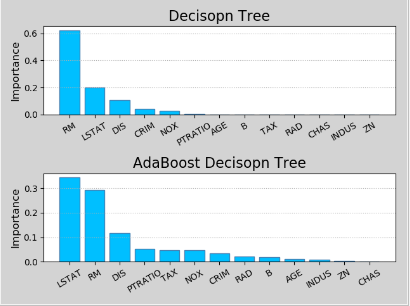
import sklearn.datasets as sd
import sklearn.utils as su
import sklearn.tree as st
import sklearn.ensemble as se
import sklearn.metrics as sm
boston = sd.load_boston()
print(boston.data.shape)  # (506, 13),506个样本,13个特征
print(boston.feature_names)  #['CRIM' 'ZN' 'INDUS' 'CHAS' 'NOX' 'RM' 'AGE' 'DIS' 'RAD' 'TAX' 'PTRATIO' 'B' 'LSTAT']
print(boston.target.shape) # (506,)
x, y = su.shuffle(boston.data, boston.target, random_state=7)  # 打乱顺序
train_size = int(len(x)*0.8)  # 用80%的数据作为训练,20%的数据作为测试
train_x, test_x, train_y, test_y = x[:train_size], x[train_size:], y[:train_size], y[train_size:]
# 决策树对象
model = st.DecisionTreeRegressor(max_depth=4)
model.fit(train_x, train_y)
pred_test_y = model.predict(test_x)
print(sm.r2_score(test_y, pred_test_y))  # 0.820256088941
# n_estimators=决策树的个数
model = se.AdaBoostRegressor(st.DecisionTreeRegressor(max_depth=4),n_estimators=400,random_state=7)
model.fit(train_x, train_y)
pred_test_y = model.predict(test_x)
print(sm.r2_score(test_y, pred_test_y))  # 0.907096311719
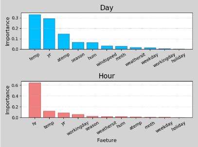
特征重要性:决策树模型在构建树状结构时,优先选择对输出结果影响最大,即可产生最大信息熵减少量的特征进行子表划分,因此该模型可以按照
特征的重要程度进行排序,即特征重要性序列。不同的模型因算法不同,所得到的特征重要性序列也会有所不同。另外,训练数据的细化程度也会影
响模型对特征重要性的判断
import matplotlib.pyplot as mp
import sklearn.datasets as sd
import sklearn.utils as su
import sklearn.tree as st
import sklearn.ensemble as se
import sklearn.metrics as sm
import numpy as np
boston = sd.load_boston()
x, y = su.shuffle(boston.data, boston.target, random_state=7)  # 打乱顺序
feature_names = boston.feature_names
train_size = int(len(x)*0.8)  # 用80%的数据作为训练,20%的数据作为测试
train_x, test_x, train_y, test_y = x[:train_size], x[train_size:], y[:train_size], y[train_size:]
# 决策树对象
model = st.DecisionTreeRegressor(max_depth=4)
model.fit(train_x, train_y)
fi_dt = model.feature_importances_
print(fi_dt)
pred_test_y = model.predict(test_x)
# n_estimators=决策树的个数
model = se.AdaBoostRegressor(st.DecisionTreeRegressor(max_depth=4),n_estimators=400,random_state=7)
model.fit(train_x, train_y)
pred_test_y = model.predict(test_x)
fi_ab = model.feature_importances_
print(fi_ab)
mp.figure('Feature Importance', facecolor='lightgray')
mp.subplot(211)
mp.title('Decisopn Tree', fontsize=16)
mp.ylabel('Importance', fontsize=12)
mp.tick_params(labelsize=10)
mp.grid(axis='y', linestyle=':')
sorted_indices = fi_dt.argsort()[::-1]
pos = np.arange(len(sorted_indices))
mp.bar(pos, fi_dt[sorted_indices], facecolor='deepskyblue', edgecolor='steelblue')
mp.xticks(pos, feature_names[sorted_indices], rotation=30)
mp.subplot(212)
mp.title('AdaBoost Decisopn Tree', fontsize=16)
mp.ylabel('Importance', fontsize=12)
mp.tick_params(labelsize=10)
mp.grid(axis='y', linestyle=':')
sorted_indices = fi_ab.argsort()[::-1]
pos = np.arange(len(sorted_indices))
mp.bar(pos, fi_ab[sorted_indices], facecolor='deepskyblue', edgecolor='steelblue')
mp.xticks(pos, feature_names[sorted_indices], rotation=30)
mp.tight_layout()
mp.show()
import csv
import numpy as np
import matplotlib.pyplot as mp
import sklearn.utils as su
import sklearn.ensemble as se
import sklearn.metrics as sm
with open('../data/bike_day.csv', 'r') as f:
    reader = csv.reader(f)
    x, y = [], []
    for row in reader:
        x.append(row[2:13])
        y.append(row[-1])
fn_dy = np.array(x[0])
x = np.array(x[1:], dtype=float)
y = np.array(y[1:], dtype=float)
x, y = su.shuffle(x, y, random_state=7)
train_size = int(len(x)*0.9)
train_x, test_x, train_y, test_y = x[:train_size], x[train_size:], y[:train_size], y[train_size:]
model = se.RandomForestRegressor(max_depth=10, n_estimators=1000, random_state=7, min_samples_split=2)
model.fit(train_x, train_y)
fi_dy = model.feature_importances_
print(fi_dy)
pred_test_y = model.predict(test_x)
print(sm.r2_score(test_y, pred_test_y))
with open('../data/bike_hour.csv', 'r') as f:
    reader = csv.reader(f)
    x, y = [], []
    for row in reader:
        x.append(row[2:13])
        y.append(row[-1])
fn_hr = np.array(x[0])
x = np.array(x[1:], dtype=float)
y = np.array(y[1:], dtype=float)
x, y = su.shuffle(x, y, random_state=7)
train_size = int(len(x)*0.9)
train_x, test_x, train_y, test_y = x[:train_size], x[train_size:], y[:train_size], y[train_size:]
model = se.RandomForestRegressor(max_depth=10, n_estimators=1000, random_state=7, min_samples_split=2)
model.fit(train_x, train_y)
fi_hr = model.feature_importances_
print(fi_hr)
pred_test_y = model.predict(test_x)
print(sm.r2_score(test_y, pred_test_y))
mp.figure('Feature Importance', facecolor='lightgray')
mp.subplot(211)
mp.title('Day', fontsize=16)
mp.ylabel('Importance', fontsize=12)
mp.tick_params(labelsize=10)
mp.grid(axis='y', linestyle=':')
sorted_indices = fi_dy.argsort()[::-1]
pos = np.arange(len(sorted_indices))
mp.bar(pos, fi_dy[sorted_indices], facecolor='deepskyblue', edgecolor='steelblue')
mp.xticks(pos, fn_dy[sorted_indices], rotation=30)
mp.subplot(212)
mp.title('Hour', fontsize=16)
mp.xlabel('Faeture', fontsize=12)
mp.ylabel('Importance', fontsize=12)
mp.tick_params(labelsize=10)
mp.grid(axis='y', linestyle=':')
sorted_indices = fi_hr.argsort()[::-1]
pos = np.arange(len(sorted_indices))
mp.bar(pos, fi_hr[sorted_indices], facecolor='lightcoral', edgecolor='indianred')
mp.xticks(pos, fn_hr[sorted_indices], rotation=30)
mp.tight_layout()
mp.show()
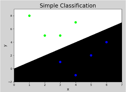
七、简单分类
x1 x2 -> y
3 1 0
2 5 1
1 8 1
6 4 0
5 2 0
3 5 1
4 7 1
4 -1 0
模型:if x1 < x2 then y = 1
if x1 > x2 then y = 0
2 9 ? ->1
7 3 ? ->0
import numpy as np
import matplotlib.pyplot as mp
x = np.array([
    [3, 1],
    [2, 5],
    [1, 8],
    [6, 4],
    [5, 2],
    [3, 5],
    [4, 7],
    [4, -1]])
y = np.array([0, 1, 1, 0, 0, 1, 1, 0])
# 画分界线,左右边界和步长,上下边界和步长
l, r, h = x[:, 0].min()-1, x[:, 0].max()+1, 0.005
b, t, v = x[:, 1].min()-1, x[:, 1].max()+1, 0.005
# 网格化
grid_x = np.meshgrid(np.arange(l, r, h), np.arange(b, t, v))
# 扁平化
flat_x = np.c_[grid_x[0].ravel(), grid_x[1].ravel()]
flat_y = np.zeros(len(flat_x), dtype=int)
flat_y[flat_x[:, 0] < flat_x[:, 1]] = 1
grid_y = flat_y.reshape(grid_x[0].shape)
mp.figure('Simple Classification', facecolor='lightgray')
mp.title('Simple Classification', fontsize=20)
mp.xlabel('x', fontsize=14)
mp.ylabel('y', fontsize=14)
mp.tick_params(labelsize=10)
mp.pcolormesh(grid_x[0], grid_x[1], grid_y, cmap='gray')
mp.scatter(x[:, 0], x[:, 1], c=y, cmap='brg', s=60)
mp.show()
八、逻辑回归
x1 x2 -> y
y = w0 + w1x1 +w2x2
1
y = ---------------
1 + e^-(w0 + w1x1 +w2x2)
在[0.1-0.5]之间视为0,(0.5-0.9]视为1
model = lm.LogisticRegression(solver='liblinear',C=正则强度) # liblinear表示w0 + w1x1 +w2x2
fit训练/predict预测
import numpy as np
import matplotlib.pyplot as mp
import sklearn.linear_model as lm
x = np.array([
    [3, 1],
    [2, 5],
    [1, 8],
    [6, 4],
    [5, 2],
    [3, 5],
    [4, 7],
    [4, -1]])
y = np.array([0, 1, 1, 0, 0, 1, 1, 0])
model = lm.LogisticRegression(solver='liblinear', C=1)
model.fit(x, y)
# 画分界线,左右边界和步长,上下边界和步长
l, r, h = x[:, 0].min()-1, x[:, 0].max()+1, 0.005
b, t, v = x[:, 1].min()-1, x[:, 1].max()+1, 0.005
# 网格化
grid_x = np.meshgrid(np.arange(l, r, h), np.arange(b, t, v))
# 扁平化
flat_x = np.c_[grid_x[0].ravel(), grid_x[1].ravel()]
flat_y = model.predict(flat_x)
grid_y = flat_y.reshape(grid_x[0].shape)
mp.figure('Logistic Classification', facecolor='lightgray')
mp.title('Logistic Classification', fontsize=20)
mp.xlabel('x', fontsize=14)
mp.ylabel('y', fontsize=14)
mp.tick_params(labelsize=10)
mp.pcolormesh(grid_x[0], grid_x[1], grid_y, cmap='gray')
mp.scatter(x[:, 0], x[:, 1], c=y, cmap='brg', s=60)
mp.show()
import numpy as np
import matplotlib.pyplot as mp
import sklearn.linear_model as lm
# 多元分类
x = np.array([
    [4, 7],
    [3.5, 8],
    [3.1, 6.2],
    [0.5, 1],
    [1, 2],
    [1.2, 1.9],
    [6, 2],
    [5.7, 1.5],
    [5.4, 2.2]])
y = np.array([0, 0, 0, 1, 1, 1, 2, 2, 2])
model = lm.LogisticRegression(solver='liblinear', C=100)
model.fit(x, y)
# 画分界线,左右边界和步长,上下边界和步长
l, r, h = x[:, 0].min()-1, x[:, 0].max()+1, 0.005
b, t, v = x[:, 1].min()-1, x[:, 1].max()+1, 0.005
# 网格化
grid_x = np.meshgrid(np.arange(l, r, h), np.arange(b, t, v))
# 扁平化
flat_x = np.c_[grid_x[0].ravel(), grid_x[1].ravel()]
flat_y = model.predict(flat_x)
grid_y = flat_y.reshape(grid_x[0].shape)
mp.figure('Logistic Classification', facecolor='lightgray')
mp.title('Logistic Classification', fontsize=20)
mp.xlabel('x', fontsize=14)
mp.ylabel('y', fontsize=14)
mp.tick_params(labelsize=10)
mp.pcolormesh(grid_x[0], grid_x[1], grid_y, cmap='gray')
mp.scatter(x[:, 0], x[:, 1], c=y, cmap='brg', s=60)
mp.show()
九、朴素贝叶斯分类
P(A):A事件发生的概率
P(A,B):A和B两个事件同时发生的概率,联合概率
P(A|B):在B事件发生的条件下A事件发生的概率,条件概率
贝叶斯定理:P(A,B) = P(B)*P(A|B)
P(B,A) = P(A)*P(B|A)
P(B)*P(A|B) = P(A)*P(B|A)
P(A)P(B|A)
P(A|B) = -------------
P(B)
朴素:条件独立,所有的特征值彼此没有任何依赖性。
