第三节 矩阵乘法和逆
矩阵乘法和逆
矩阵乘法
- 第一种方法(一般方法):
假设有矩阵等式\(C=AB\):
\({ \left[ {{\left. \begin{array}{*{20}{l}} {a\mathop{{}}\nolimits_{{11}}\text{ }\text{ }a\mathop{{}}\nolimits_{{12}}\text{ }\text{ }a\mathop{{}}\nolimits_{{13}}\text{ }\text{ }a\mathop{{}}\nolimits_{{14}}}\\ {a\mathop{{}}\nolimits_{{21}}\text{ }\text{ }a\mathop{{}}\nolimits_{{22}}\text{ }\text{ }a\mathop{{}}\nolimits_{{23}}\text{ }\text{ }a\mathop{{}}\nolimits_{{24}}}\\ {a\mathop{{}}\nolimits_{{31}}\text{ }\text{ }a\mathop{{}}\nolimits_{{32}}\text{ }\text{ }a\mathop{{}}\nolimits_{{33}}\text{ }\text{ }a\mathop{{}}\nolimits_{{34}}}\\ {a\mathop{{}}\nolimits_{{41}}\text{ }\text{ }a\mathop{{}}\nolimits_{{42}}\text{ }\text{ }a\mathop{{}}\nolimits_{{43}}\text{ }\text{ }a\mathop{{}}\nolimits_{{44}}} \end{array} \right] }{ \left[ {{\left. \begin{array}{*{20}{l}} {b\mathop{{}}\nolimits_{{11}}\text{ }\text{ }b\mathop{{}}\nolimits_{{12}}\text{ }\text{ }b\mathop{{}}\nolimits_{{13}}\text{ }\text{ }b\mathop{{}}\nolimits_{{14}}}\\ {b\mathop{{}}\nolimits_{{21}}\text{ }\text{ }b\mathop{{}}\nolimits_{{22}}\text{ }\text{ }b\mathop{{}}\nolimits_{{23}}\text{ }\text{ }b\mathop{{}}\nolimits_{{24}}}\\ {b\mathop{{}}\nolimits_{{31}}\text{ }\text{ }b\mathop{{}}\nolimits_{{32}}\text{ }\text{ }b\mathop{{}}\nolimits_{{33}}\text{ }\text{ }b\mathop{{}}\nolimits_{{34}}}\\ {b\mathop{{}}\nolimits_{{41}}\text{ }\text{ }b\mathop{{}}\nolimits_{{42}}\text{ }\text{ }b\mathop{{}}\nolimits_{{43}}\text{ }\text{ }b\mathop{{}}\nolimits_{{44}}} \end{array} \right] }={ \left[ {{\left. \begin{array}{*{20}{l}} {c\mathop{{}}\nolimits_{{11}}\text{ }\text{ }c\mathop{{}}\nolimits_{{12}}\text{ }\text{ }c\mathop{{}}\nolimits_{{13}}\text{ }\text{ }c\mathop{{}}\nolimits_{{14}}}\\ {c\mathop{{}}\nolimits_{{21}}\text{ }\text{ }c\mathop{{}}\nolimits_{{22}}\text{ }\text{ }c\mathop{{}}\nolimits_{{23}}\text{ }\text{ }c\mathop{{}}\nolimits_{{24}}}\\ {c\mathop{{}}\nolimits_{{31}}\text{ }\text{ }c\mathop{{}}\nolimits_{{32}}\text{ }\text{ }c\mathop{{}}\nolimits_{{33}}\text{ }\text{ }c\mathop{{}}\nolimits_{{34}}}\\ {c\mathop{{}}\nolimits_{{41}}\text{ }\text{ }c\mathop{{}}\nolimits_{{42}}\text{ }\text{ }c\mathop{{}}\nolimits_{{43}}\text{ }\text{ }c\mathop{{}}\nolimits_{{44}}} \end{array} \right] }}\right. }}\right. }}\right. }\)
则\({c\mathop{{}}\nolimits_{{ij}}}=矩阵A的行i∙矩阵B的列j\)
即:\({c\mathop{{}}\nolimits_{{ij}}=a\mathop{{}}\nolimits_{{i1}}b\mathop{{}}\nolimits_{{1j}}+a\mathop{{}}\nolimits_{{i2}}b\mathop{{}}\nolimits_{{2j}}+a\mathop{{}}\nolimits_{{i3}}b\mathop{{}}\nolimits_{{3j}}+\text{ …… }+a\mathop{{}}\nolimits_{{ik}}b\mathop{{}}\nolimits_{{kj}}={\mathop{ \sum }\limits_{{k=1}}^{{n}}{a\mathop{{}}\nolimits_{{ik}}b\mathop{{}}\nolimits_{{kj}}}}}\)
从上面的式子看出,要使两个矩阵能够相乘,矩阵\(A\)的列要等于矩阵\(B\)的行。并且可以看出矩阵\(C\)的行是由矩阵\(A\)决定,列是由矩阵\(B\)决定,
即一个\(m∗n\)的\(A\)矩阵,和一个\(n∗p\)的\(B\)矩阵相乘,将得到一个\(m∗p\)的矩阵\(C\)
-
第二种方法(整列考虑):
用矩阵\(A\)乘以矩阵\(B\)的每一列(即矩阵乘以向量,方法第一节提到过),得到的矩阵\(C\)的每一列都是矩阵\(A\)各列的线性组合
-
第三种方法(整行考虑):B
用矩阵\(A\)的每一行乘以矩阵\(B\)(即向量乘以矩阵,方法第一节提到过),得到的矩阵\(C\)的每一行都是矩阵\(B\)各行的线性组合
回到上节留下的问题
\({\begin{array}{*{20}{l}}
{E\mathop{{}}\nolimits_{{32}} \left( E\mathop{{}}\nolimits_{{21}}A \left) =U\right. \right. }\\
{E\mathop{{}}\nolimits_{{32}}={ \left[ {{\left. \begin{array}{*{20}{l}}
{1\text{ }\text{ }0\text{ }\text{ }0}\\
{0\text{ }\text{ }1\text{ }\text{ }0}\\
{0\text{ }-4\text{ }1}
\end{array} \right] }\text{ }\text{ }\text{ }\text{ }E\mathop{{}}\nolimits_{{21}}={ \left[ {{\left. \begin{array}{*{20}{l}}
{1\text{ }\text{ }0\text{ }\text{ }0}\\
{-3\text{ }1\text{ }\text{ }0}\\
{0\text{ }\text{ }0\text{ }\text{ }1}
\end{array} \right] }}\right. }}\right. }}\\
{E\mathop{{}}\nolimits_{{32}}E\mathop{{}}\nolimits_{{21}}={ \left[ {{\left. \begin{array}{*{20}{l}}
{1\text{ }\text{ }0\text{ }\text{ }0}\\
{0\text{ }\text{ }1\text{ }\text{ }0}\\
{0\text{ }\text{ }0\text{ }\text{ }1}
\end{array} \right] }=I}\right. }}
\end{array}}\)
即\(EA=I\)
-
乘法小技巧
在网上找到的图
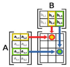
把矩阵\(B\)的位置向上移,这样做乘法就不会在计算时串行
矩阵的逆
如果矩阵\(A\)满足:\({{A\mathop{{}}\nolimits^{{-1}}}A=AA\mathop{{}}\nolimits^{{-1}}=I}\),那么矩阵\(A\)就是可逆的
\({A\mathop{{}}\nolimits^{{-1}}}\)表示矩阵\(A\)的逆矩阵。\(I\)表示单位矩阵,因为单位矩阵是方阵,所以可逆矩阵都是方阵
接下来观察不可逆的矩阵,例:
\({A={ \left[ {{\left. \begin{array}{*{20}{l}} {1\text{ }\text{ }3}\\ {2\text{ }\text{ }6} \end{array} \right] }}\right. }}\)
-
那么矩阵\(A\)为什么是不可逆的?
-
矩阵\(A\)的行列式等于\(0\)(后面会讲行列式)
-
刚才提到,如果矩阵可逆,那么它与逆矩阵相乘结果是单位矩阵,刚才讲到矩阵相乘,如果从整列考虑,结果应该与矩阵\(A\)成线性关系,但矩阵\(A\)的每一列不可能与单位矩阵的每一列成线性关系
-
如果能找到一个向量\(X\),使\(AX=0(X \neq 0)\),那么这个矩阵就是不可逆的,比如:
\({A={ \left[ {{\left. \begin{array}{*{20}{l}} {1\text{ }\text{ }3}\\ {2\text{ }\text{ }6} \end{array} \right] }{ \left[ {{\left. \begin{array}{*{20}{l}} {3}\\ {-1} \end{array} \right] }={ \left[ {{\left. \begin{array}{*{20}{l}} {0}\\ {0} \end{array} \right] }}\right. }}\right. }}\right. }}\)
如果矩阵\(A\)是可逆矩阵,那么向量\(X\)一定为\(0\),所以要求\(X \neq 0\)
-
-
怎么求矩阵的逆?
例:\({\begin{array}{*{20}{l}} {{ \left[ {{\left. \begin{array}{*{20}{l}} {1\text{ }\text{ }3}\\ {2\text{ }\text{ }7} \end{array} \right] }{{ \left[ {{\left. \begin{array}{*{20}{l}} {a\text{ }\text{ }b}\\ {c\text{ }\text{ }d} \end{array} \right] }}\right. }={ \left[ {{\left. \begin{array}{*{20}{l}} {1\text{ }\text{ }0}\\ {0\text{ }\text{ }1} \end{array} \right] }}\right. }}}\right. }}\\ {\text{ }\text{ }\text{ }\text{ }\text{ }\text{ }\text{ }\text{ }AA\mathop{{}}\nolimits^{{-1}}=I} \end{array}}\)
按照上节学习的消元法解线性方程组,要解这两个方程组
\({\begin{array}{*{20}{l}} {{ \left[ {{\left. \begin{array}{*{20}{l}} {1\text{ }\text{ }3}\\ {2\text{ }\text{ }7} \end{array} \right] }{{ \left[ {{\left. \begin{array}{*{20}{l}} {a}\\ {c} \end{array} \right] }}\right. }={ \left[ {{\left. \begin{array}{*{20}{l}} {1}\\ {0} \end{array} \right] }}\right. }}}\right. }}\\ {{ \left[ {{\left. \begin{array}{*{20}{l}} {1\text{ }\text{ }3}\\ {2\text{ }\text{ }7} \end{array} \right] }{{ \left[ {{\left. \begin{array}{*{20}{l}} {b}\\ {d} \end{array} \right] }}\right. }={ \left[ {{\left. \begin{array}{*{20}{l}} {0}\\ {1} \end{array} \right] }}\right. }}}\right. }} \end{array}}\)
利用高斯-若尔当消元法(Gauss-Jordan Elimination),没必要一个一个解这两个方程组,可以把系数矩阵和由两个右侧向量组成的矩阵再组成一个大矩阵
\({ \left[ {{\left. \begin{array}{*{20}{l}} {1\text{ }\text{ }3\text{ }\text{ }1\text{ }\text{ }0}\\ {2\text{ }\text{ }7\text{ }\text{ }0\text{ }\text{ }1} \end{array} \right] }}\right. } \xrightarrow { \left( 2,1 \right) }{ \left[ {{\left. \begin{array}{*{20}{l}} {1\text{ }\text{ }3\text{ }\text{ }\text{ }\text{ }1\text{ }\text{ }0}\\ {0\text{ }\text{ }1\text{ }\text{ }-2\text{ }\text{ }1} \end{array} \right] }}\right. }\)
按照上节消元法,到这一步就完了,高斯-若尔当消元法增加了一步,消去(1,2),则结果为:
\({ \left[ {{\left. \begin{array}{*{20}{l}} {1\text{ }\text{ }0\text{ }\text{ }7\text{ }\text{ }-3}\\ {0\text{ }\text{ }1\text{ }-2\text{ }\text{ }\text{ }1} \end{array} \right] }}\right. }\)
可以检验\({ \left[ {{\left. \begin{array}{*{20}{l}} {\text{ }7\text{ }\text{ }-3}\\ {-2\text{ }\text{ }\text{ }1} \end{array} \right] }}\right. }\)就是矩阵\(A\)的逆矩阵
对于可逆矩阵,\(EA=I,AA\mathop{{}}\nolimits^{{-1}}=I\),那么\(E=A\mathop{{}}\nolimits^{{-1}}\),即高斯-若尔当消元法所引入的一些\(E\)的积就是\(A\)的逆矩阵