python—sift特征提取

一、SIFT提出的目的和意义

二、SIFT的特征简介

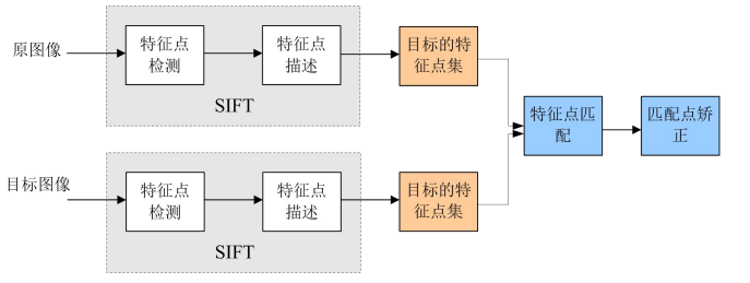
三、SIFT算法实现步骤简述

四、图像集

五、匹配地理标记图像

 

• 代码
• 结果截图
• 小结 

 

六、SIFT算法代码实现

• 代码
• 结果截图
• 小结 

七、图像全景拼接RANSAC

八、SIFT实验总结

九、实验遇到的问题

 

一、SIFT提出的目的和意义

1999年David G.Lowe教授总结了基于特征不变技术的检测方法，在图像尺度空间基础上，提出了对图像缩放、旋转保持不变性的图像局部特征描述算子－SIFT（尺度不变特征变换），该算法在2004年被加以完善。

 

二、SIFT的特征简介

SIFT算法可以解决的问题

1.  目标的旋转、缩放、平移（RST）
2. 图像仿射/投影变换（视点viewpoint）
3. 弱光照影响（illumination）
4. 部分目标遮挡（occlusion）
5. 杂物场景（clutter）
6. 噪声

 

 三、SIFT算法实现步骤简述

SIFT算法的实质可以归为在不同尺度空间上查找特征点（关键点）的问题。SIFT算法实现特征匹配主要有三个流程，1、提取关键点；2、对关键点附加详细的信息（局部特征），即描述符；3、通过特征点（附带上特征向量的关键点）的两两比较找出相互匹配的若干对特征点，建立景物间的对应关系。

 

                                                                         图1

需要配置vfleat安装包

使用开源工具包 VLFeat 提供的二进制文件来计算图像的 SIFT特征 。这里附上VLFeat 工具包链接http://www.vlfeat.org/ 
操作步骤：
1.把vlfeat文件夹下win64中的sift.exe和vl.dll这两个文件复制到项目的文件夹中

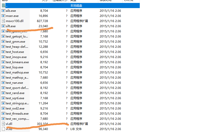
2.修改PCV文件夹内的(我的PCV位置为D:\Anaconda2\Lib\site-packages\PCV))文件夹里面的localdescriptors文件夹中的sift.py文件，用记事本打开，修改其中的cmmd内的路径cmmd=str(r"D:\new\sift.exe“+imagename+” --output="+resultname+" "+params) （路径是你项目文件夹中的sift.exe的路径）一定要在括号里加上r。

 

 

 

四、图像集

一共19 张图像

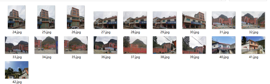
                                                                                                                     图2

 

五、匹配地理标记图像        

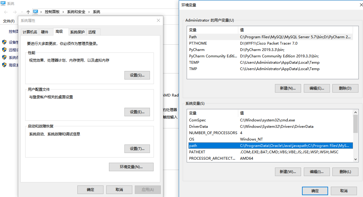
 1、做此实验我们需用pydot工具包中的GraphViz，可以点击https://graphviz.gitlab.io/_pages/Download/Download_windows.html下载安装包，安装步骤如下：

      配置环境: 保存graphviz安装时，一定要记住保存路径，方便找到你的安装包安装中的gvedit.exe的位置，我的是C:\Program Files (x86)\Graphviz2.38\bin

把gvedit.exe发送到桌面快捷方式，然后去系统里点击高级系统设置->点击环境变量->点击系统变量的path选择编辑->输入C:\Program Files (x86)\Graphviz2.38\bin，之后就确定保存。

 

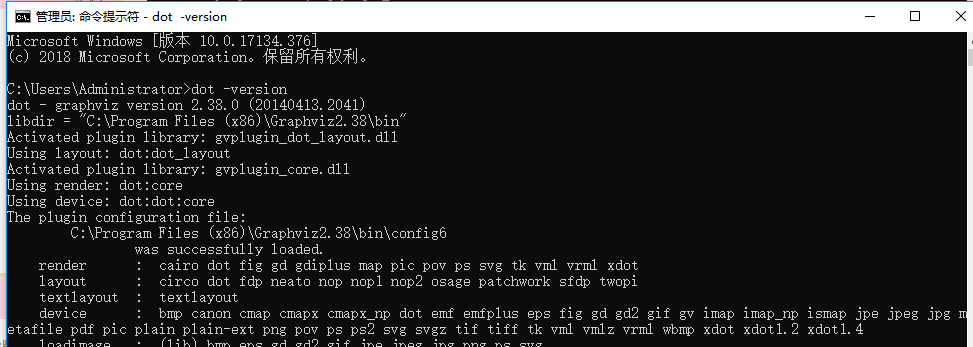
 接下来是验证环境配置是否成功，输入dot -version命令，成功如下：

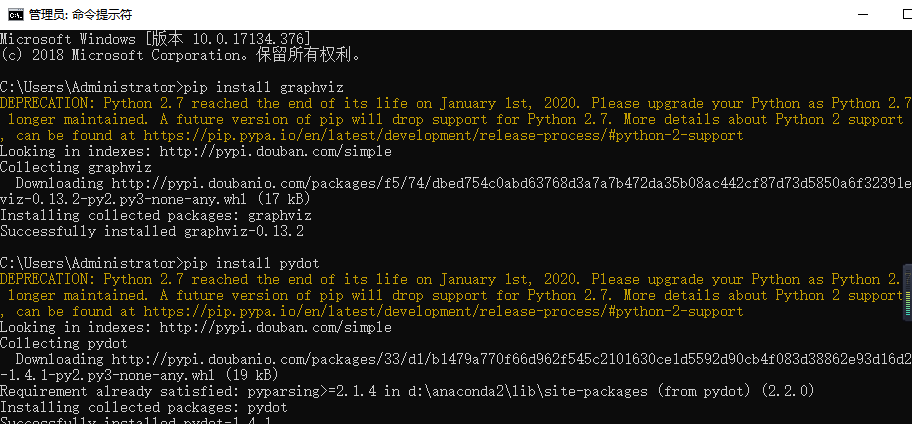
然后依次执行以下命令：

pip install graphviz

pip install pydot

 

成功如下：

 d

 2、实验代码：

# -*- coding: utf-8 -*-
from pylab import *
from PIL import Image
from PCV.localdescriptors import sift
from PCV.tools import imtools
import pydot
 
""" This is the example graph illustration of matching images from Figure 2-10.
To download the images, see ch2_download_panoramio.py."""
 
#download_path = "panoimages"  # set this to the path where you downloaded the panoramio images
#path = "/FULLPATH/panoimages/"  # path to save thumbnails (pydot needs the full system path)
 
#download_path = "F:\\dropbox\\Dropbox\\translation\\pcv-notebook\\data\\panoimages"  # set this to the path where you downloaded the panoramio images
#path = "F:\\dropbox\\Dropbox\\translation\\pcv-notebook\\data\\panoimages\\"  # path to save thumbnails (pydot needs the full system path)
download_path = "D:/new"
path = "D:/new"
# list of downloaded filenames
imlist = imtools.get_imlist(download_path)
nbr_images = len(imlist)
 
# extract features
featlist = [imname[:-3] + 'sift' for imname in imlist]
for i, imname in enumerate(imlist):
    sift.process_image(imname, featlist[i])
 
matchscores = zeros((nbr_images, nbr_images))
 
for i in range(nbr_images):
    for j in range(i, nbr_images):  # only compute upper triangle
        print 'comparing ', imlist[i], imlist[j]
        l1, d1 = sift.read_features_from_file(featlist[i])
        l2, d2 = sift.read_features_from_file(featlist[j])
        matches = sift.match_twosided(d1, d2)
        nbr_matches = sum(matches > 0)
        print 'number of matches = ', nbr_matches
        matchscores[i, j] = nbr_matches
print "The match scores is: %d", matchscores
 
#np.savetxt(("../data/panoimages/panoramio_matches.txt",matchscores)
 
# copy values
for i in range(nbr_images):
    for j in range(i + 1, nbr_images):  # no need to copy diagonal
        matchscores[j, i] = matchscores[i, j]
 
threshold = 2  # min number of matches needed to create link
 
g = pydot.Dot(graph_type='graph')  # don't want the default directed graph
 
for i in range(nbr_images):
    for j in range(i + 1, nbr_images):
        if matchscores[i, j] > threshold:
            # first image in pair
            im = Image.open(imlist[i])
            im.thumbnail((100, 100))
            filename = path + str(i) + '.png'
            im.save(filename)  # need temporary files of the right size
            g.add_node(pydot.Node(str(i), fontcolor='transparent', shape='rectangle', image=filename))
 
            # second image in pair
            im = Image.open(imlist[j])
            im.thumbnail((100, 100))
            filename = path + str(j) + '.png'
            im.save(filename)  # need temporary files of the right size
            g.add_node(pydot.Node(str(j), fontcolor='transparent', shape='rectangle', image=filename))
 
            g.add_edge(pydot.Edge(str(i), str(j)))
g.write_png('protect2.png')

3、结果截图：

         

 

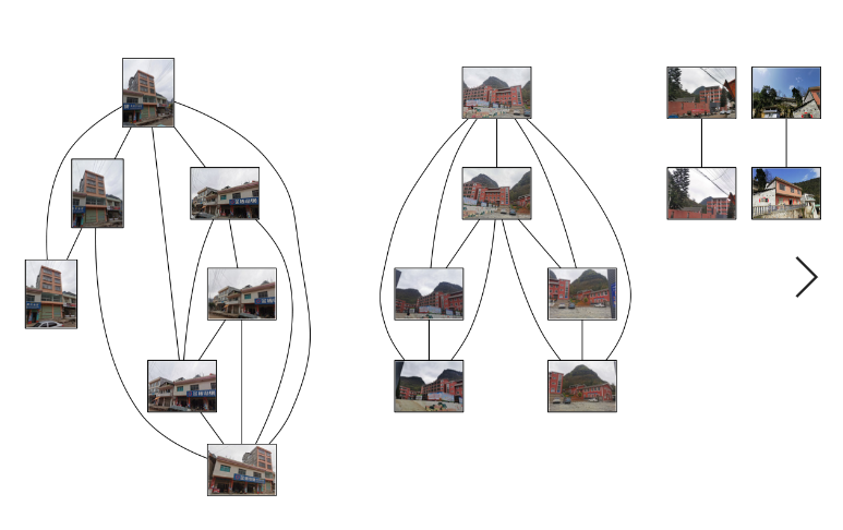
 实验小结：图像集一共有十九张图片，运行出来只有十七张图片，我拍摄的照片范围过小，只选择了六个地点拍摄，没有显示出来的两张图片是跟以上图片没有太多相似的特征点的。显示出来的第一个连线的部分，是在同一个位置拍摄，只是从不同的角度，但是提取出来的特征点匹配度很高，说明了sift算法角度不变性，还有色彩影响不是很大，并且只要有一点特征点匹配度的图片就会相连起来，第二部分和第三部分依然如此。

                                                                    

六、SIFT算法代码实现

1、单张图片的sift特征提取、Harris角点提取、用圆圈表示SIFT特征尺度提取

代码：

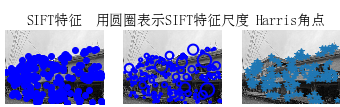
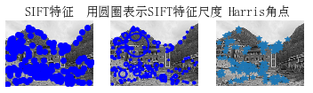
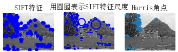
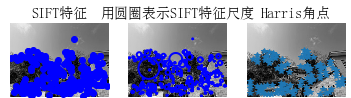
# -*- coding: utf-8 -*-
from PIL import Image
from pylab import *
from PCV.localdescriptors import sift
from PCV.localdescriptors import harris

# 添加中文字体支持
from matplotlib.font_manager import FontProperties
font = FontProperties(fname=r"c:\windows\fonts\SimSun.ttc", size=14)

imname = 'siftt/24.jpg'
im = array(Image.open(imname).convert('L'))
sift.process_image(imname, '24.sift')
l1, d1 = sift.read_features_from_file('24.sift')

figure()
gray()
subplot(131)
sift.plot_features(im, l1, circle=False)
title(u'SIFT特征',fontproperties=font)
subplot(132)
sift.plot_features(im, l1, circle=True)
title(u'用圆圈表示SIFT特征尺度',fontproperties=font)

# 检测harris角点
harrisim = harris.compute_harris_response(im)

subplot(133)
filtered_coords = harris.get_harris_points(harrisim, 6, 0.1)
imshow(im)
plot([p[1] for p in filtered_coords], [p[0] for p in filtered_coords], '*')
axis('off')
title(u'Harris角点',fontproperties=font)

show()

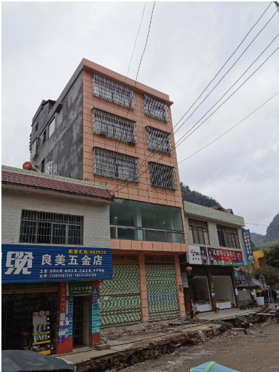
原图

运行结果：

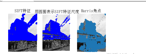
小结：由图看出，sift算法检测出来的特征点比harris角点算法检测出的角点多。sift算法测出来的特征点大多数都是重合的。

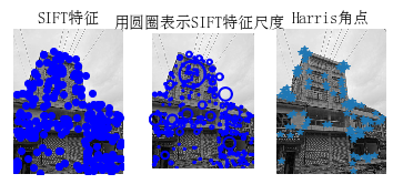
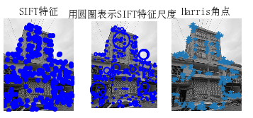
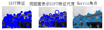
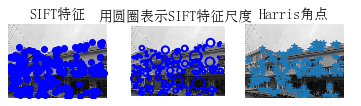
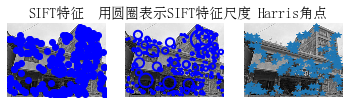
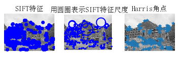
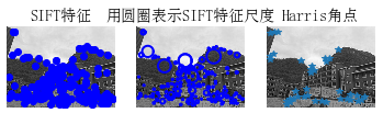
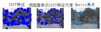
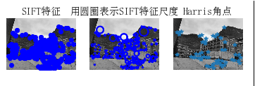
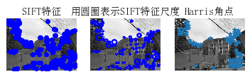
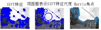
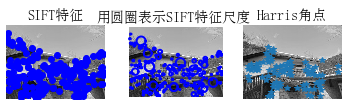
 2、图像集里的所有图像的sift特征提取

 代码：

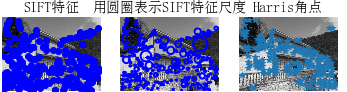
# -*- coding: utf-8 -*-
from PIL import Image
from pylab import *
from PCV.localdescriptors import sift
from PCV.localdescriptors import harris
from PCV.tools.imtools import get_imlist # 导入原书的PCV模块

# 添加中文字体支持
from matplotlib.font_manager import FontProperties
font = FontProperties(fname=r"c:\windows\fonts\SimSun.ttc", size=14)

# 获取project2_data文件夹下的图片文件名(包括后缀名)
filelist = get_imlist('siftt/')

for infile in filelist: # 对文件夹下的每张图片进行如下操作
    print(infile) # 输出文件名
    
    im = array(Image.open(infile).convert('L'))
    sift.process_image(infile, 'infile.sift')
    l1, d1 = sift.read_features_from_file('infile.sift')
    i=1
    
    figure(i)
    i=i+1
    gray()
    
    subplot(131)
    sift.plot_features(im, l1, circle=False)
    title(u'SIFT特征',fontproperties=font)
    
    subplot(132)
    sift.plot_features(im, l1, circle=True)
    title(u'用圆圈表示SIFT特征尺度',fontproperties=font)
    
    # 检测harris角点
    harrisim = harris.compute_harris_response(im)
    
    subplot(133)
    filtered_coords = harris.get_harris_points(harrisim, 6, 0.1)
    imshow(im)
    plot([p[1] for p in filtered_coords], [p[0] for p in filtered_coords], '*')
    axis('off')
    title(u'Harris角点',fontproperties=font)
    
    show()

 

结果截图：

 

 

 

 

 

 

 

 

 

 

 

 

 

 

 

 

 

 

 

 

 

 

 

 

 

 

 

 

 

 

 

 

 

 

 

3、两张图片，计算sift特征匹配结果

代码：

# -*- coding: utf-8 -*-
from PIL import Image
from pylab import *
from numpy import *
import os

def process_image(imagename, resultname, params="--edge-thresh 10 --peak-thresh 5"):
    """ 处理一幅图像，然后将结果保存在文件中"""
    if imagename[-3:] != 'pgm':
        #创建一个pgm文件
        im = Image.open(imagename).convert('L')
        im.save('tmp.pgm')
        imagename ='tmp.pgm'
    cmmd = str("sift "+imagename+" --output="+resultname+" "+params)
    os.system(cmmd)
    print 'processed', imagename, 'to', resultname
    
def read_features_from_file(filename):
    """读取特征属性值，然后将其以矩阵的形式返回"""
    f = loadtxt(filename)
    return f[:,:4], f[:,4:] #特征位置，描述子
    
def write_featrues_to_file(filename, locs, desc):
    """将特征位置和描述子保存到文件中"""
    savetxt(filename, hstack((locs,desc)))
    
def plot_features(im, locs, circle=False):
    """显示带有特征的图像
       输入：im（数组图像），locs（每个特征的行、列、尺度和朝向）"""
       
    def draw_circle(c,r):
        t = arange(0,1.01,.01)*2*pi
        x = r*cos(t) + c[0]
        y = r*sin(t) + c[1]
        plot(x, y, 'b', linewidth=2)
        
    imshow(im)
    if circle:
        for p in locs:
            draw_circle(p[:2], p[2])
    else:
        plot(locs[:,0], locs[:,1], 'ob')
    axis('off')
    
def match(desc1, desc2):
    """对于第一幅图像中的每个描述子，选取其在第二幅图像中的匹配
    输入：desc1(第一幅图像中的描述子)，desc2(第二幅图像中的描述子)"""
    desc1 = array([d/linalg.norm(d) for d in desc1])
    desc2 = array([d/linalg.norm(d) for d in desc2])
    dist_ratio = 0.6
    desc1_size = desc1.shape
    matchscores = zeros((desc1_size[0],1),'int')
    desc2t = desc2.T #预先计算矩阵转置
    for i in range(desc1_size[0]):
        dotprods = dot(desc1[i,:],desc2t) #向量点乘
        dotprods = 0.9999*dotprods
        # 反余弦和反排序，返回第二幅图像中特征的索引
        indx = argsort(arccos(dotprods))
        #检查最近邻的角度是否小于dist_ratio乘以第二近邻的角度
        if arccos(dotprods)[indx[0]] < dist_ratio * arccos(dotprods)[indx[1]]:
            matchscores[i] = int(indx[0])
    return matchscores
    
def match_twosided(desc1, desc2):
    """双向对称版本的match()"""
    matches_12 = match(desc1, desc2)
    matches_21 = match(desc2, desc1)
    ndx_12 = matches_12.nonzero()[0]
    # 去除不对称的匹配
    for n in ndx_12:
        if matches_21[int(matches_12[n])] != n:
            matches_12[n] = 0
    return matches_12
    
def appendimages(im1, im2):
    """返回将两幅图像并排拼接成的一幅新图像"""
    #选取具有最少行数的图像，然后填充足够的空行
    rows1 = im1.shape[0]
    rows2 = im2.shape[0]
    if rows1 < rows2:
        im1 = concatenate((im1, zeros((rows2-rows1,im1.shape[1]))),axis=0)
    elif rows1 >rows2:
        im2 = concatenate((im2, zeros((rows1-rows2,im2.shape[1]))),axis=0)
    return concatenate((im1,im2), axis=1)
    
def plot_matches(im1,im2,locs1,locs2,matchscores,show_below=True):
    """ 显示一幅带有连接匹配之间连线的图片
        输入：im1, im2(数组图像), locs1,locs2（特征位置）,matchscores(match()的输出)，
        show_below（如果图像应该显示在匹配的下方）
    """
    im3=appendimages(im1, im2)
    if show_below:
        im3=vstack((im3, im3))
    imshow(im3)
    cols1 = im1.shape[1]
    for i in range(len(matchscores)):
        if matchscores[i]>0:
            plot([locs1[i,0],locs2[matchscores[i,0],0]+cols1], [locs1[i,1],locs2[matchscores[i,0],1]],'c')
    axis('off')
    
im1f = 'siftt/25.jpg'
im2f = 'siftt/26.jpg'

im1 = array(Image.open(im1f))
im2 = array(Image.open(im2f))

process_image(im1f, 'out_sift_1.txt')
l1,d1 = read_features_from_file('out_sift_1.txt')
figure()
gray()
subplot(121)
plot_features(im1, l1, circle=False)

process_image(im2f, 'out_sift_2.txt')
l2,d2 = read_features_from_file('out_sift_2.txt')
subplot(122)
plot_features(im2, l2, circle=False)

matches = match_twosided(d1, d2)
print '{} matches'.format(len(matches.nonzero()[0]))

figure()
gray()
plot_matches(im1, im2, l1, l2, matches, show_below=True)
show()

 

结果截图：

 

 

 

 

 

 

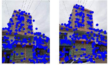
 小结：用siftt算法提取两张图的特征点，然后双向匹配两张图片的描述子，用线将两幅图相匹配的描述子相连，连的线越多，说明这两幅图的匹配度越高，两幅图越相似。

 4、给定一张图片，输出匹配度最高的三张图片

代码：

# -*- coding: utf-8 -*-
from PIL import Image
from pylab import *
from numpy import *
import os
from PCV.tools.imtools import get_imlist # 导入原书的PCV模块
import matplotlib.pyplot as plt # plt 用于显示图片
import matplotlib.image as mpimg # mpimg 用于读取图片

def process_image(imagename, resultname, params="--edge-thresh 10 --peak-thresh 5"):
    """ 处理一幅图像，然后将结果保存在文件中"""
    if imagename[-3:] != 'pgm':
        #创建一个pgm文件
        im = Image.open(imagename).convert('L')
        im.save('tmp.pgm')
        imagename ='tmp.pgm'
    cmmd = str("sift "+imagename+" --output="+resultname+" "+params)
    os.system(cmmd)
    print 'processed', imagename, 'to', resultname
    
def read_features_from_file(filename):
    """读取特征属性值，然后将其以矩阵的形式返回"""
    f = loadtxt(filename)
    return f[:,:4], f[:,4:] #特征位置，描述子
    
def write_featrues_to_file(filename, locs, desc):
    """将特征位置和描述子保存到文件中"""
    savetxt(filename, hstack((locs,desc)))
    
def plot_features(im, locs, circle=False):
    """显示带有特征的图像
       输入：im（数组图像），locs（每个特征的行、列、尺度和朝向）"""
       
    def draw_circle(c,r):
        t = arange(0,1.01,.01)*2*pi
        x = r*cos(t) + c[0]
        y = r*sin(t) + c[1]
        plot(x, y, 'b', linewidth=2)
        
    imshow(im)
    if circle:
        for p in locs:
            draw_circle(p[:2], p[2])
    else:
        plot(locs[:,0], locs[:,1], 'ob')
    axis('off')
    
def match(desc1, desc2):
    """对于第一幅图像中的每个描述子，选取其在第二幅图像中的匹配
    输入：desc1(第一幅图像中的描述子)，desc2(第二幅图像中的描述子)"""
    desc1 = array([d/linalg.norm(d) for d in desc1])
    desc2 = array([d/linalg.norm(d) for d in desc2])
    dist_ratio = 0.6
    desc1_size = desc1.shape
    matchscores = zeros((desc1_size[0],1),'int')
    desc2t = desc2.T #预先计算矩阵转置
    for i in range(desc1_size[0]):
        dotprods = dot(desc1[i,:],desc2t) #向量点乘
        dotprods = 0.9999*dotprods
        # 反余弦和反排序，返回第二幅图像中特征的索引
        indx = argsort(arccos(dotprods))
        #检查最近邻的角度是否小于dist_ratio乘以第二近邻的角度
        if arccos(dotprods)[indx[0]] < dist_ratio * arccos(dotprods)[indx[1]]:
            matchscores[i] = int(indx[0])
    return matchscores
    
def match_twosided(desc1, desc2):
    """双向对称版本的match()"""
    matches_12 = match(desc1, desc2)
    matches_21 = match(desc2, desc1)
    ndx_12 = matches_12.nonzero()[0]
    # 去除不对称的匹配
    for n in ndx_12:
        if matches_21[int(matches_12[n])] != n:
            matches_12[n] = 0
    return matches_12
    
def appendimages(im1, im2):
    """返回将两幅图像并排拼接成的一幅新图像"""
    #选取具有最少行数的图像，然后填充足够的空行
    rows1 = im1.shape[0]
    rows2 = im2.shape[0]
    if rows1 < rows2:
        im1 = concatenate((im1, zeros((rows2-rows1,im1.shape[1]))),axis=0)
    elif rows1 >rows2:
        im2 = concatenate((im2, zeros((rows1-rows2,im2.shape[1]))),axis=0)
    return concatenate((im1,im2), axis=1)
    
def plot_matches(im1,im2,locs1,locs2,matchscores,show_below=True):
    """ 显示一幅带有连接匹配之间连线的图片
        输入：im1, im2(数组图像), locs1,locs2（特征位置）,matchscores(match()的输出)，
        show_below（如果图像应该显示在匹配的下方）
    """
    im3=appendimages(im1, im2)
    if show_below:
        im3=vstack((im3, im3))
    imshow(im3)
    cols1 = im1.shape[1]
    for i in range(len(matchscores)):
        if matchscores[i]>0:
            plot([locs1[i,0],locs2[matchscores[i,0],0]+cols1], [locs1[i,1],locs2[matchscores[i,0],1]],'c')
    axis('off')
    
# 获取project2_data文件夹下的图片文件名(包括后缀名)
filelist = get_imlist('project2_data/')

# 输入的图片
im1f = '23.jpg'
im1 = array(Image.open(im1f))
process_image(im1f, 'out_sift_1.txt')
l1, d1 = read_features_from_file('out_sift_1.txt')

i=0
num = [0]*30    #存放匹配值
for infile in filelist: # 对文件夹下的每张图片进行如下操作
    im2 = array(Image.open(infile))
    process_image(infile, 'out_sift_2.txt')
    l2, d2 = read_features_from_file('out_sift_2.txt')
    matches = match_twosided(d1, d2)
    num[i] = len(matches.nonzero()[0])
    i=i+1
    print '{} matches'.format(num[i-1])  #输出匹配值
    
i=1
figure()
while i<4: #循环三次，输出匹配最多的三张图片
    index=num.index(max(num))
    print index, filelist[index]
    lena = mpimg.imread(filelist[index])  # 读取当前匹配最大值的图片
    # 此时 lena 就已经是一个 np.array 了，可以对它进行任意处理
    # lena.shape  # (512, 512, 3)
    subplot(1,3,i)
    plt.imshow(lena)  # 显示图片
    plt.axis('off')  # 不显示坐标轴
    num[index] = 0  #将当前最大值清零
    i=i+1
show()

 

结果截图：

给定的图片

 

 

输出的图片

 

小结：通过用给定的图匹配图像集中的每张图片的描述子，然后用线与图像集中的图片的描述子相连，匹配度最高的图片就会被输出。

 七、图像全景拼接RANSAC

7.1 RANSAC算法原理

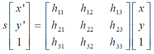
OpenCV中滤除误匹配对采用RANSAC算法寻找一个最佳单应性矩阵H，矩阵大小为3×3。RANSAC目的是找到最优的参数矩阵使得满足该矩阵的数据点个数最多，通常令h33=1来归一化矩阵。由于单应性矩阵有8个未知参数，至少需要8个线性方程求解，对应到点位置信息上，一组点对可以列出两个方程，则至少包含4组匹配点对。

                    

 

 

 RANSAC算法从匹配数据集中随机抽出4个样本并保证这4个样本之间不共线，计算出单应性矩阵，然后利用这个模型测试 

                    

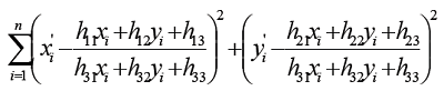
所有数据，并计算满足这个模型数据点的个数与投影误差(即代价函数)，若此模型为最优模型，则对应的代价函数最小。

7.2 RANSAC算法步骤 

  1. 随机从数据集中随机抽出4个样本数据 (此4个样本之间不能共线)，计算出变换矩阵H，记为模型M；

  2. 计算数据集中所有数据与模型M的投影误差，若误差小于阈值，加入内点集 I ；

  3. 如果当前内点集 I 元素个数大于最优内点集 I_best , 则更新 I_best = I，同时更新迭代次数k ;

  4. 如果迭代次数大于k,则退出 ; 否则迭代次数加1，并重复上述步骤；

  注：迭代次数k在不大于最大迭代次数的情况下，是在不断更新而不是固定的；p为置信度，一般取0.995；w为"内点"的比例 ; m为计算模型所需要的最少样本数=4；

7.3 RANSAC 基本假设

测试的数据都是由"局外点"组成的，建立模型，局外点是不能适应该模型的数据，也就是不合适该模型的局外点就是噪声。

7.4  RANSAC 局外点产生的原因

A、噪声的极值

B、错误的测量方法

C、对数据的错误假设

7.5实验代码

 

from pylab import *
from PIL import Image
import warp
import homography
import sift
 
# set paths to data folder
featname = ['D:/new/jia/' + str(i + 1) + '.sift' for i in range(3)]
imname = ['D:/new/jia/' + str(i + 1) + '.jpg' for i in range(3)]
 
# extract features and match
l = {}
d = {}
for i in range(3):
    sift.process_image(imname[i], featname[i])
    l[i], d[i] = sift.read_features_from_file(featname[i])
 
matches = {}
for i in range(2):
    matches[i] = sift.match(d[i + 1], d[i])
 
# visualize the matches (Figure 3-11 in the book)
for i in range(2):
    im1 = array(Image.open(imname[i]))
    im2 = array(Image.open(imname[i + 1]))
    figure()
    sift.plot_matches(im2, im1, l[i + 1], l[i], matches[i], show_below=True)
 
 
# function to convert the matches to hom. points
def convert_points(j):
    ndx = matches[j].nonzero()[0]
    fp = homography.make_homog(l[j + 1][ndx, :2].T)
    ndx2 = [int(matches[j][i]) for i in ndx]
    tp = homography.make_homog(l[j][ndx2, :2].T)
 
    # switch x and y - TODO this should move elsewhere
    fp = vstack([fp[1], fp[0], fp[2]])
    tp = vstack([tp[1], tp[0], tp[2]])
    return fp, tp
 
 
# estimate the homographies
model = homography.RansacModel()
 
fp,tp = convert_points(1)
H_12 = homography.H_from_ransac(fp,tp,model)[0] #im 1 to 2
 
fp,tp = convert_points(0)
H_01 = homography.H_from_ransac(fp,tp,model)[0] #im 0 to 1
 
 
# warp the images
delta = 1000 # for padding and translation
 
im1 = array(Image.open(imname[1]), "uint8")
im2 = array(Image.open(imname[2]), "uint8")
im_12 = warp.panorama(H_12,im1,im2,delta,delta)
 
im1 = array(Image.open(imname[0]), "f")
im_02 = warp.panorama(dot(H_12,H_01),im1,im_12,delta,delta)
 
figure()
imshow(array(im_02, "uint8"))
axis('off')
show()

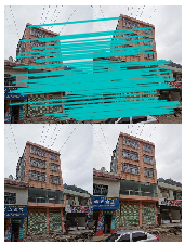
7.6结果截图

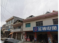
单一的环境图片

 

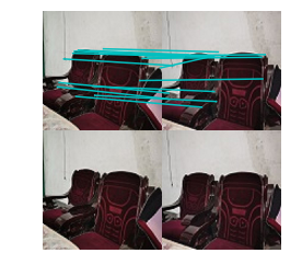
分析：我拍摄的是四张图片，环境很单一，同一个场景，不同的角度，由结果截图看出前面一张图片的拼接点较多，从第二张看出删除点较为明显，一看就可以看出来那些点被删除了，删除后觉得看到的连线比较清晰，连接的线条变少。

 

 

 

 

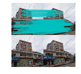
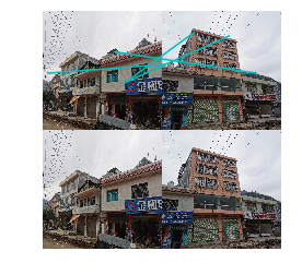
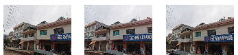
分析：这组图片是同一个地点拍的，环境比较丰富，从不同的角度拍摄，第一张图片跟第二张的不同点相当的明显，第一张的连线很多，拼接的效果很成功，连线很多，看出有重复点，覆盖匹配点，第二张的图片相似点较少，连线也不多，说明了，相似度高的匹配程度就高，拼接效果也好，相似度低的就相反。

 

 

7.7遇到的问题

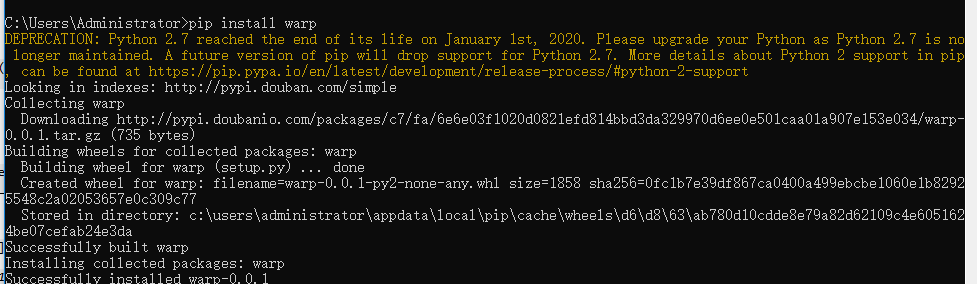
因为运行之前没有导入包，就产生了错误，然后我就导入了warp包

 报错

 Arrays cannot be empty 

矩阵为空，我就重新改了图像的像素，提取sift特征

然后由报错

 did not meet fit acceptance criteria 

这是因为图片的水平落差比较大，我们得再拍一组照片。改了图片的下高速，图片的像素都改成一样，不能太大也不能太小，我改成的是600*600.

 

八、SIFT实验总结

1、sift算法提取特征点稳定，不会因为光照、旋转、尺度等因素而改变图像的特征点。

2、图像的尺度越大，图像就会越模糊。

3、sift算法可以对多张图像进行快速的、准确的关键点匹配，产生大量的特征点，可以适用于生活中的很多运用。

4、sift算法提取的特征点会有重叠。

5、在用sift算法提取特征时，应该降低图片的像素，像素过高会导致运行时间过长或失败。

 

九、实验遇到的问题

出现的问题：1、运行代码时出现这样的错误：

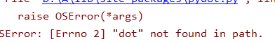
在D:\Anaconda2\Lib\site-packages目录中找到pydot.py ，用记事本打开，把self.prog = 'dot‘改成self.prog = r'C:\Program Files (x86)\Graphviz2.38\bin\dot.exe'，保存，关掉运行软件再打开就可以了。

 2、运行代码出现这样的结果

 

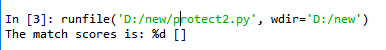
 我用的项目的路径，出现以上报错，把路径改成了图片的路径，图片的后缀改成.jpg就可以了。

 3、因为图片像素过高，运行时间会过长，结果一直出不来，还以为是代码出来了错误，但是不报错，想着可能是照片是自己拍的，像素过高了，就去降低了图片的像素，运行速率变快，结果就出来了。