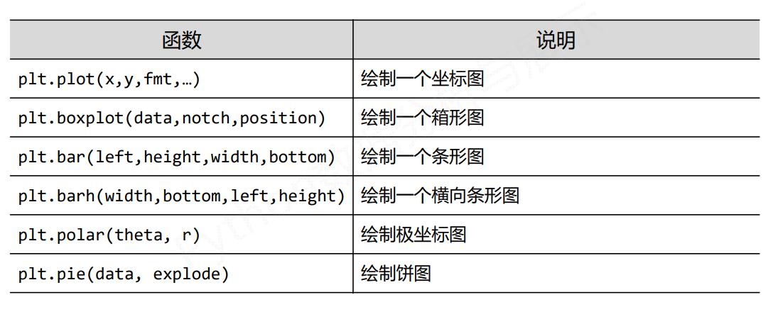
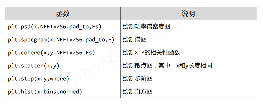
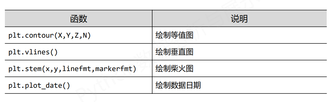
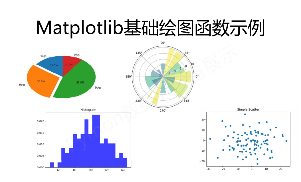
Pyplot基础图表函数
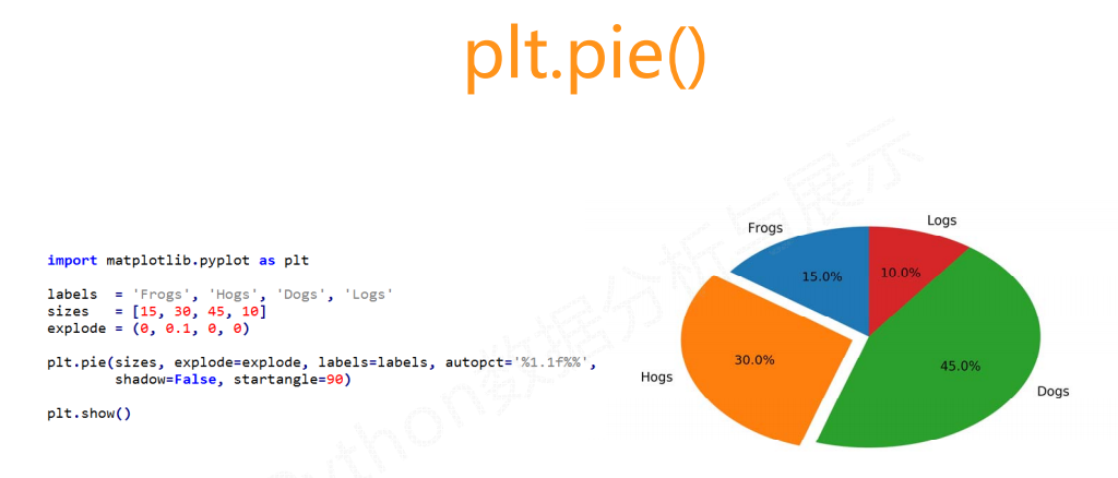
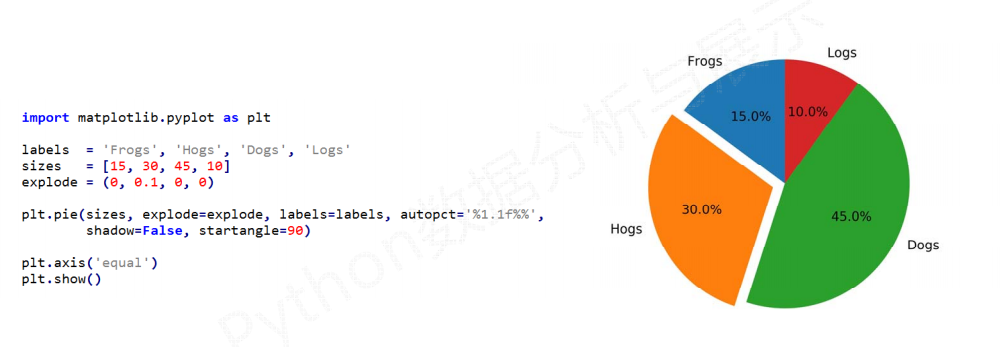
Pyplot饼图的绘制:
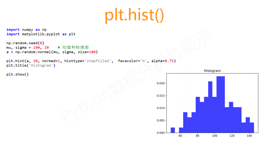
Pyplot直方图的绘制:

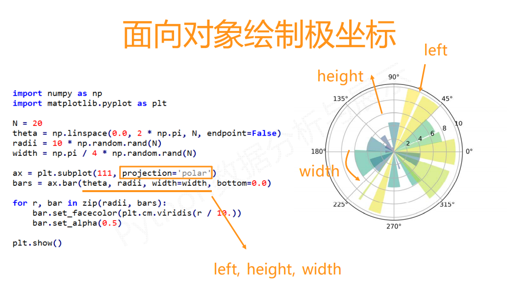
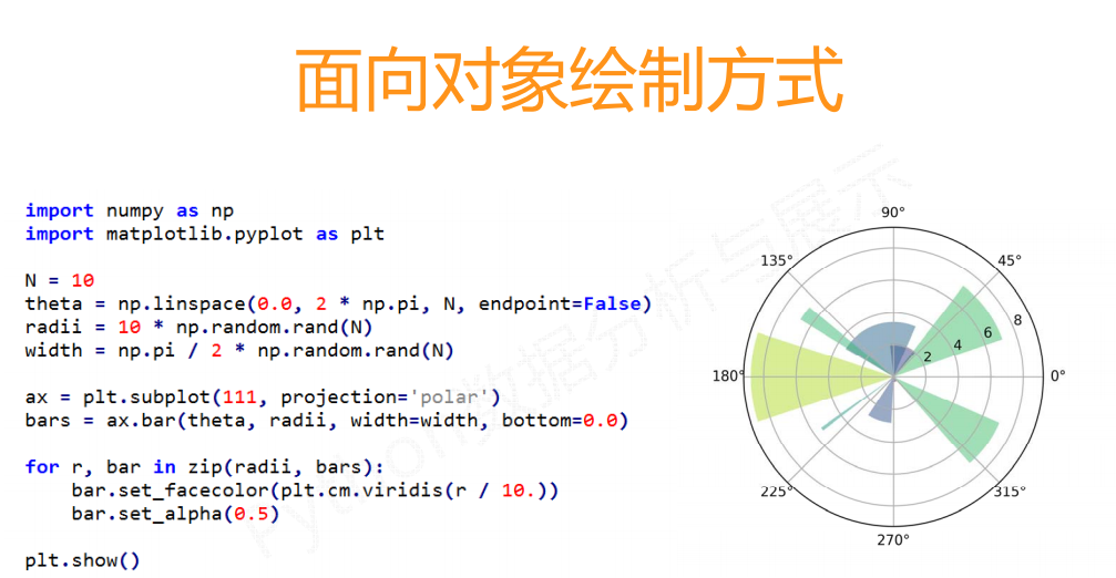
Pyplot极坐标图的绘制:
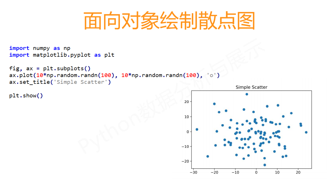
Pyplot散点图的绘制:
单元小结:

import numpy as np
import matplotlib.pyplot as plt
from scipy.io import wavfile

rate_h, hstrain= wavfile.read(r"H1_Strain.wav","rb")
rate_l, lstrain= wavfile.read(r"L1_Strain.wav","rb")
#reftime, ref_H1 = np.genfromtxt('GW150914_4_NR_waveform_template.txt').transpose()
reftime, ref_H1 = np.genfromtxt('wf_template.txt').transpose() #使用python123.io下载文件

htime_interval = 1/rate_h
ltime_interval = 1/rate_l
fig = plt.figure(figsize=(12, 6))

# 丢失信号起始点
htime_len = hstrain.shape[0]/rate_h
htime = np.arange(-htime_len/2, htime_len/2 , htime_interval)
plth = fig.add_subplot(221)
plth.plot(htime, hstrain, 'y')
plth.set_xlabel('Time (seconds)')
plth.set_ylabel('H1 Strain')
plth.set_title('H1 Strain')

ltime_len = lstrain.shape[0]/rate_l
ltime = np.arange(-ltime_len/2, ltime_len/2 , ltime_interval)
pltl = fig.add_subplot(222)
pltl.plot(ltime, lstrain, 'g')
pltl.set_xlabel('Time (seconds)')
pltl.set_ylabel('L1 Strain')
pltl.set_title('L1 Strain')

pltref = fig.add_subplot(212)
pltref.plot(reftime, ref_H1)
pltref.set_xlabel('Time (seconds)')
pltref.set_ylabel('Template Strain')
pltref.set_title('Template')
fig.tight_layout()

plt.savefig("Gravitational_Waves_Original.png")
plt.show()
plt.close(fig)


【推荐】编程新体验,更懂你的AI,立即体验豆包MarsCode编程助手
【推荐】凌霞软件回馈社区,博客园 & 1Panel & Halo 联合会员上线
【推荐】抖音旗下AI助手豆包,你的智能百科全书,全免费不限次数
【推荐】轻量又高性能的 SSH 工具 IShell:AI 加持,快人一步