观影数据集2

5 筛选数据

 

#票房、预算、受欢迎程度、评分为0的数据应该去除；

#评分人数过低的电影，评分不具有统计意义，这里筛选评分人数大于50的数据。

df.describe()

df = df[(df.vote_count >= 50) &(df.budget * df.revenue * df.popularity * df.vote_average !=0)].reset_index(drop = 'True')

df

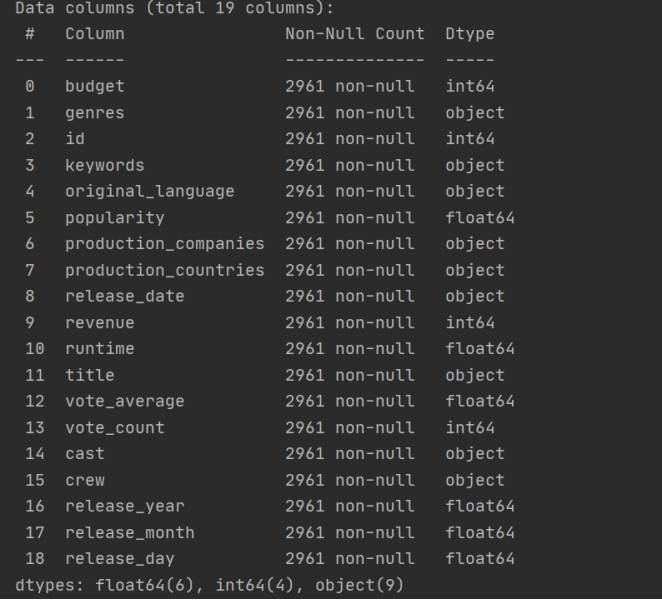
df.info()

 

 

 

 

使用数据分析师最喜欢的一个语法：

 

票房、预算、受欢迎程度、评分为 0  的数据应该去除；

评分人数过低的电影，评分不具有统计意义，筛选评分人数大于    50   的数据。

 

此时剩余    2961   条数据，包含 19 个字段。

 

6 json 数据转换

 

**说明：**genres,keywords,production_companies,production_countries,cast,crew 这 6 列都是

 

json 数据，需要处理为列表进行分析。处理方法：

json 本身为字符串类型，先转换为字典列表，再将字典列表转换为，以’,'分割的字符串

 

 

json_column = ['genres', 'keywords', 'production_companies', 'production_countries', 'cast', 'crew']

 

# 1-json本身为字符串类型，先转换为字典列表

for i in json_column:

    df[i] = df[i].apply(json.loads)

 

 

# 提取name

# 2-将字典列表转换为以','分割的字符串

def get_name(x):

    return ','.join([i['name'] for i in x])

 

 

df['cast'] = df['cast'].apply(get_name)

 

 

# 提取derector

def get_director(x):

    for i in x:

        if i['job'] == 'Director':

            return i['name']

 

 

df['crew'] = df['crew'].apply(get_director)

 

for j in json_column[0:4]:

    df[j] = df[j].apply(get_name)

 

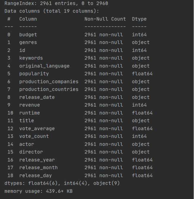
# 重命名

rename_dict = {'cast': 'actor', 'crew': 'director'}

df.rename(columns=rename_dict, inplace=True)

df.info()

df.head(5)

 

 

 

7 数据备份

org_df = df.copy()

df.reset_index().to_csv("TMDB_5000_Movie_Backup.csv")

 

8 数据分析

 

8.1 why

 

想要探索影响票房的因素，从电影市场趋势，观众喜好类型，电影导演，发行时间，评分与关键词等维度着手，给从业者提供合适的建议。

8.2 what

 

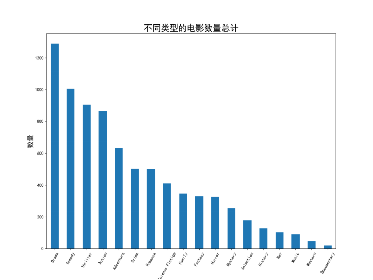
8.2.1 电影类型：定义一个集合，获取所有的电影类型

 

注意到集合中存在多余的元素：空的单引号，所以需要去除。

 

 

genre = set()

for i in df['genres'].str.split(','): # 去掉字符串之间的分隔符，得到单个电影类型

    genre = set().union(i,genre)    # 集合求并集

    # genre.update(i) #或者使用update方法

 

print(genre)

#注意到genre集合中存在多余的元素：空的单引号，所以需要去除

genre.discard('') # 去除多余的元素

genre

 

 

 

 

8.2.1.1 电影类型数量（绘制条形图）

 

 

 

 

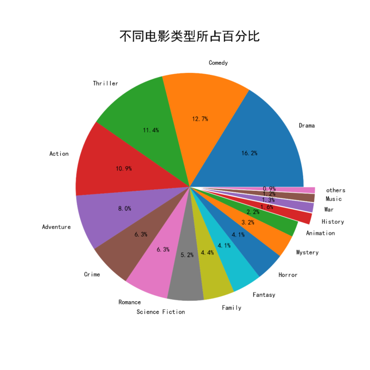
8.2.1.2 电影类型占比（绘制饼图）

 

 

 

 

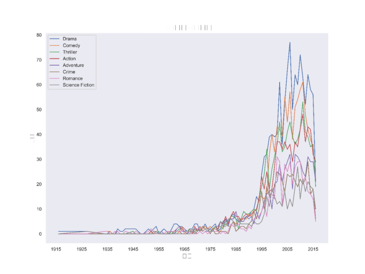
8.2.1.3 电影类型变化趋势（绘制折线图）

 

 

 

 

 

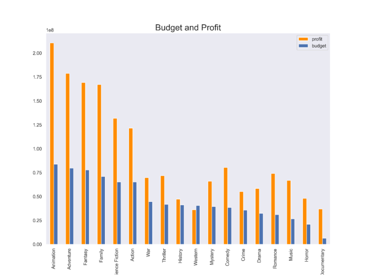
8.2.1.4 不同电影类型预算/利润（绘制组合图）

 

 

 

 

8.2.2 电影关键词（keywords 关键词分析，绘制词云图）

 

 

 

8.3 when

 

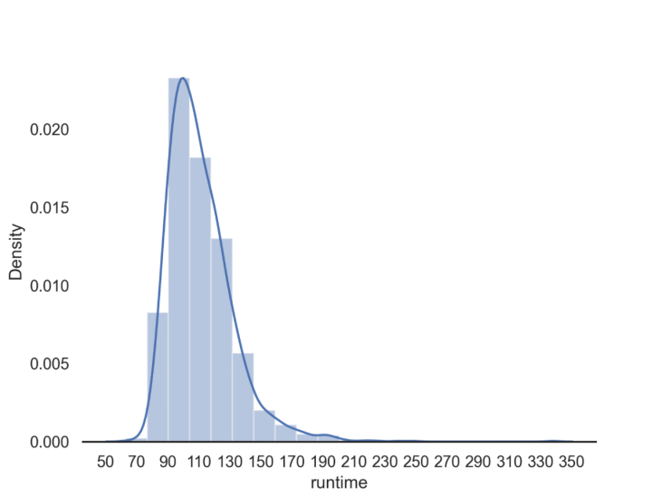
查看 runtime 的类型，发现是 object 类型，也就是字符串，所以，先进行数据转化。

 

#查看 runtime 的类型，发现是 object 类型，也就是字符串，所以，先进行数据转化。

 

print(df.runtime.head(5))

df.runtime = df.runtime.astype(float)

print(df.runtime.head(5))

 

 

 

 

 

 

 

8.3.1 电影时长（绘制电影时长直方图）

 

sns.set_style('white')

sns.distplot(df.runtime,bins = 20)

sns.despine(left = True) # 使用despine()方法来移除坐标轴，默认移除顶部和右侧坐标轴

plt.xticks(range(50,360,20))

plt.savefig('电影时长直方图.png',dpi=300)

plt.show()

 

 

 

 

 

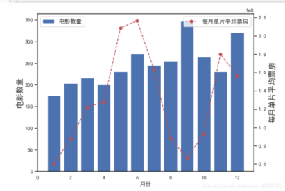
8.3.2 发行时间（绘制每月电影数量和单片平均票房）

fig = plt.figure(figsize=(8,6))

 

x = list(range(1,13))

y1 = df.groupby('release_month').revenue.size()

y2 = df.groupby('release_month').revenue.mean()# 每月单片平均票房

 

# 左轴

ax1 = fig.add_subplot(1,1,1)

plt.bar(x,y1,color='b',label='电影数量')

plt.grid(False)

ax1.set_xlabel(u'月份')# 设置x轴label ,y轴label

ax1.set_ylabel(u'每月电影数量',fontsize=16)

ax1.legend(loc=2,fontsize=12)

 

# 右轴

ax2 = ax1.twinx()

plt.plot(x,y2,'ro--',label=u'单片平均票房')

ax2.set_ylabel(u'每月单片平均票房',fontsize=16)

ax2.legend(loc=1,fontsize=12)

 

plt.rcParams['font.sans-serif'] = ['SimHei']

plt.savefig('每月电影数量和单片平均票房.png',dpi=300)

plt.rc("font",family="SimHei",size="15")

plt.show()

 

 

 

 

 

 

8.4 where

 

本数据集收集的是美国地区的电影数据，对于电影的制作公司以及制作国家，在本次的故事背景下不作分析。

8.5 who

 

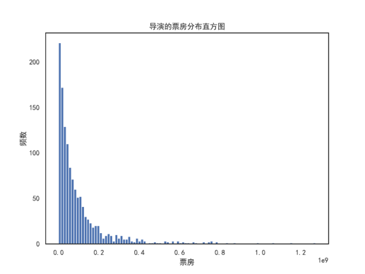
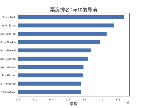
8.5.1 分析票房分布及票房 Top10 的导演

 

# 创建数据框 - 导演

director_df = pd.DataFrame()

 

director_df = df[['director','revenue','budget','vote_average']]

director_df['profit'] = (director_df['revenue']-director_df['budget'])

 

director_df = director_df.groupby(by = 'director').mean().sort_values(by='revenue',ascending = False) # 取均值

director_df.info()

 

# 绘制票房分布直方图

director_df['revenue'].plot.hist(bins=100, figsize=(8,6))

plt.xlabel('票房')

plt.ylabel('频数')

plt.title('导演的票房分布直方图')

plt.savefig('导演的票房分布直方图.png',dpi = 300)

plt.show()

 

# 票房均值Top10的导演

director_df.revenue.sort_values(ascending = True).tail(10).plot(kind='barh',figsize=(8,6))

plt.xlabel('票房',fontsize = 16)

plt.ylabel('导演',fontsize = 16)

plt.title('票房排名Top10的导演',fontsize = 20)

plt.savefig('票房排名Top10的导演.png',dpi = 300)

plt.show()

 

 

 

 

8.5.2 分析评分分布及评分 Top10 的导演

 

 

 

 

8.6 how

 

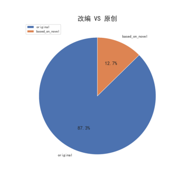
8.6.1 原创 VS 改编占比（饼图）

 

# 创建数据框

original_df = pd.DataFrame()

original_df['keywords'] = df['keywords'].str.contains('based on').map(lambda x: 1 if x else 0)

original_df['profit'] = df['revenue'] - df['budget']

original_df['budget'] = df['budget']

 

# 计算

novel_cnt = original_df['keywords'].sum() # 改编作品数量

original_cnt = original_df['keywords'].count() - original_df['keywords'].sum() # 原创作品数量

# 按照 是否原创 分组

original_df = original_df.groupby('keywords', as_index = False).mean() # 注意此处计算的是利润和预算的平均值

# 增加计数列

original_df['count'] = [original_cnt, novel_cnt]

# 计算利润率

original_df['profit_rate'] = (original_df['profit'] / original_df['budget'])*100

 

# 修改index

original_df.index = ['original', 'based_on_novel']

# 计算百分比

original_pie = original_df['count'] / original_df['count'].sum()

 

# 绘制饼图

original_pie.plot(kind='pie',label='',startangle=90,shadow=False,autopct='%2.1f%%',figsize=(8,8))

plt.title('改编 VS 原创',fontsize=20)

plt.legend(loc=2,fontsize=10)

plt.savefig('改编VS原创-饼图.png',dpi=300)

plt.show()

 

 

 

 

 

 

 

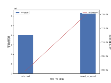
8.6.2 原创 VS 改编预算/利润率（组合图）

 

x = original_df.index

y1 = original_df.budget

y2 = original_df.profit_rate

 

fig= plt.figure(figsize = (8,6))

 

# 左轴

ax1 = fig.add_subplot(1,1,1)

plt.bar(x,y1,color='b',label='平均预算',width=0.25)

plt.xticks(rotation=0, fontsize=12)  # 更改横坐标轴名称

ax1.set_xlabel('原创 VS 改编')                   # 设置x轴label ,y轴label

ax1.set_ylabel('平均预算',fontsize=16)

ax1.legend(loc=2,fontsize=10)

 

#右轴

# 共享x轴，生成次坐标轴

ax2 = ax1.twinx()

ax2.plot(x,y2,color='r',label='平均利润率')

ax2.set_ylabel('平均利润率',fontsize=16)

ax2.legend(loc=1,fontsize=10) # loc=1,2,3,4分别表示四个角，和四象限顺序一致

 

# 将利润率坐标轴以百分比格式显示

import matplotlib.ticker as mtick

fmt='%.1f%%'

yticks = mtick.FormatStrFormatter(fmt)

ax2.yaxis.set_major_formatter(yticks)

 

plt.savefig('改编VS原创的预算以及利润率-组合图.png',dpi=300)

plt.show()

 

 

 

 

 

8.7 how much

 

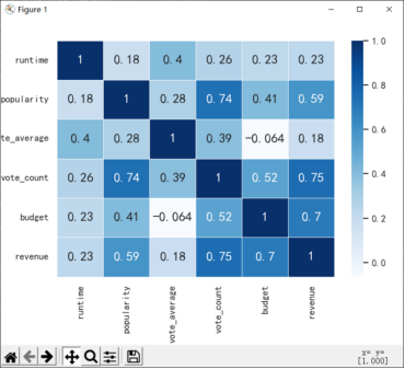
8.7.1 计算相关系数（票房相关系数矩阵）

 

revenue_corr = df[['runtime','popularity','vote_average','vote_count','budget','revenue']].corr()

 

sns.heatmap(

            revenue_corr,

            annot=True, # 在每个单元格内显示标注

            cmap="Blues", # 设置填充颜色：黄色，绿色，蓝色

            cbar=True,  # 显示color bar

            linewidths=0.5, # 在单元格之间加入小间隔，方便数据阅读

           )

plt.savefig('票房相关系数矩阵.png',dpi=300)

plt.show()

 

 

 

 

 

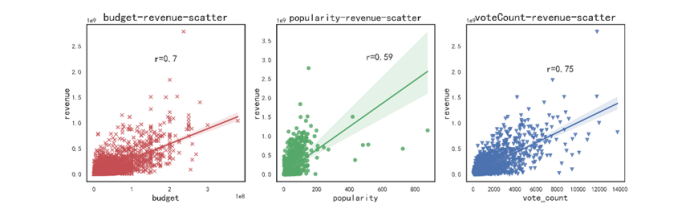
8.7.2 票房影响因素散点图

 

fig = plt.figure(figsize=(17,5))

 

ax1 = plt.subplot(1,3,1)

ax1 = sns.regplot(x='budget', y='revenue', data=df, x_jitter=.1,color='r',marker='x')

# marker: 'x','o','v','^','<'

# jitter:抖动项，表示抖动程度

ax1.text(1.6e8,2.2e9,'r=0.7',fontsize=16)

plt.title('budget-revenue-scatter',fontsize=20)

plt.xlabel('budget',fontsize=16)

plt.ylabel('revenue',fontsize=16)

 

ax2 = plt.subplot(1,3,2)

ax2 = sns.regplot(x='popularity', y='revenue', data=df, x_jitter=.1,color='g',marker='o')

ax2.text(500,3e9,'r=0.59',fontsize=16)

plt.title('popularity-revenue-scatter',fontsize=18)

plt.xlabel('popularity',fontsize=16)

plt.ylabel('revenue',fontsize=16)

 

ax3 = plt.subplot(1,3,3)

ax3 = sns.regplot(x='vote_count', y='revenue', data=df, x_jitter=.1,color='b',marker='v')

ax3.text(7000,2e9,'r=0.75',fontsize=16)

plt.title('voteCount-revenue-scatter',fontsize=20)

plt.xlabel('vote_count',fontsize=16)

plt.ylabel('revenue',fontsize=16)

plt.savefig('revenue.png',dpi=300)

plt.show()