高斯分布2

  多元高斯分布的概率密度函数如下：
\(\mathscr N(\bf{x} |\bf{\mu}, \Sigma) = \frac{1}{(2\pi)^{n/2}|\sigma|^{-1/2}}exp{\{-\frac{1}{2}(x-\mu)^{T}\Sigma^{-1}(x-\mu) \}}\)
其中，\(\bf x \in R^{n\times1}\),\(\bf \mu\)为向量均值，\(\bf \Sigma\)为协方差矩阵
【1】多元高斯分布的均值和方差证明 待补充
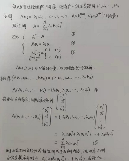
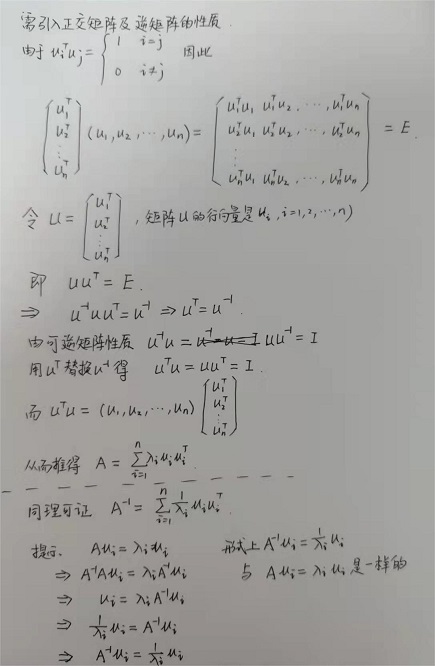
【2】假设协方差矩阵是实对称矩阵，且有n个不为0的特征值，则可以对原空间进行线性变换，使得变换后的空间各个维度上的特征向量正交。如此以来变换后的协方差矩阵就是对角矩阵。证明如下：

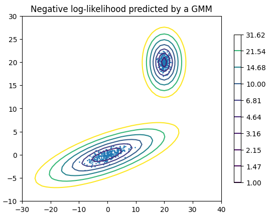
  下面是分别是使用随机生成的二维数据和老忠实泉喷发数据，绘制用高斯混合模型预测的图形

import numpy as np
import matplotlib.pyplot as plt
from matplotlib.colors import LogNorm
from sklearn import mixture

n_samples = 300

# generate random sample, two components
np.random.seed(0)

# generate spherical data centered on (20, 20)
shifted_gaussian = np.random.randn(n_samples, 2) + np.array([20, 20])

# generate zero centered stretched Gaussian data
C = np.array([[0.0, -0.7], [3.5, 0.7]])
stretched_gaussian = np.dot(np.random.randn(n_samples, 2), C)

# concatenate the two datasets into the final training set
X_train = np.vstack([shifted_gaussian, stretched_gaussian])

# fit a Gaussian Mixture Model with two components
clf = mixture.GaussianMixture(n_components=2, covariance_type="full")
clf.fit(X_train)

# display predicted scores by the model as a contour plot
x = np.linspace(-30.0, 40.0)
y = np.linspace(-10.0, 30.0)
X, Y = np.meshgrid(x, y)
XX = np.array([X.ravel(), Y.ravel()]).T
Z = -clf.score_samples(XX)
Z = Z.reshape(X.shape)

CS = plt.contour(X, Y, Z, levels=np.logspace(0, 1.5, 10))
CB = plt.colorbar(CS, shrink=0.8, extend="both")
plt.scatter(X_train[:, 0], X_train[:, 1], 0.8)

plt.title("Negative log-likelihood predicted by a GMM")
plt.axis("tight")
plt.show()

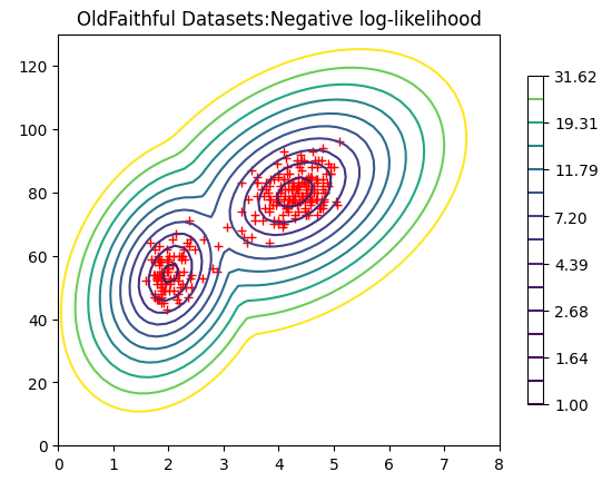
  将上述随机生成的数据替换成老忠实泉的喷发数据，横坐标是每次喷发持续的时间，纵坐标是每天喷发的间隔时间，由此绘制的图形如下：

【参考】
https://scikit-learn.org/stable/auto_examples/mixture/plot_gmm_pdf.html