机器学习之线性回归
一.分类,回归区别
- 分类:有类别,如对错:1,0;去银行贷款:贷,不贷
- 回归:和具体数值或范围相关:如:去银行贷款多少钱:10000元(在具体范围中的取值:1到1000取99)
二.有监督和无监督区别
- 有无标签进行监督,而回归就是有监督的问题,需要x1,x2特征,y标签
三.回归问题:银行贷款额度预测
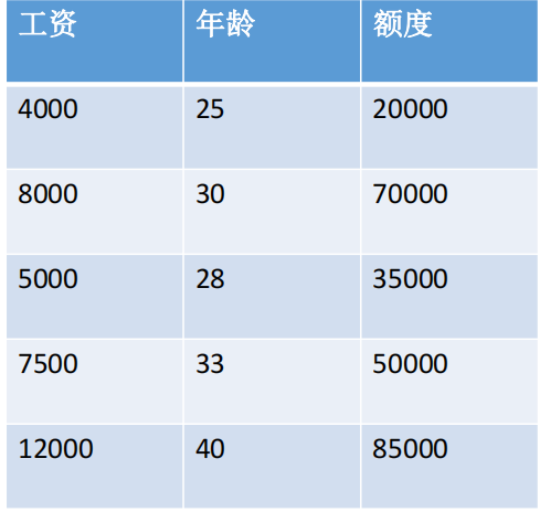
- 1.特征:年龄(x1),工资(x2)
- 2.预测:额度(y)
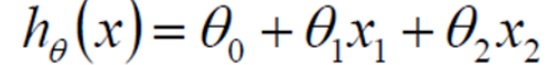
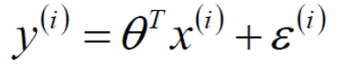
- 3.思考:x1,x2在贷款额度所占权重不同,可得公式 y=x1θ1+x2θ2,而θ1,θ2即权重,即是需要求的未知变量。
- 4.求解思路 :
- 首先:
线性方程不能满足所有的数据点只能尽可能拟合出一个平面去拟合大部分的数据点如:
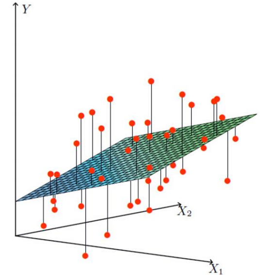
注意θ0为偏置项,其作用为控制平面上下浮动微调,去拟合大部分数据点.(微调) - 其次:
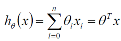
因为我们处理的数据大部分是矩阵类型的,但是上述公式中由于θ0的出现不能去拟合矩阵公式,故而增加x0,这就是为什么在数据处理时有时增加一列特征x0并且值为1
- 再其次
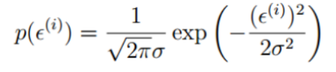
因为真实值和预测值是存在差异的,用ε表示,而ε称为误差(均值为0,方差为θ平方,独立且具有相同的分布的高斯分布)
又因为服从正态分布,故
而 可以替换为
可以替换为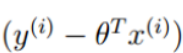 得到
得到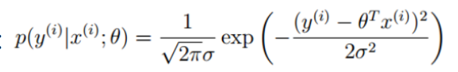 越大越好
越大越好
为什么越大越好:因为P概率是θ与x(i)组成的预测值成为y真实值的概率,所以一定是越大越好 - 再其次
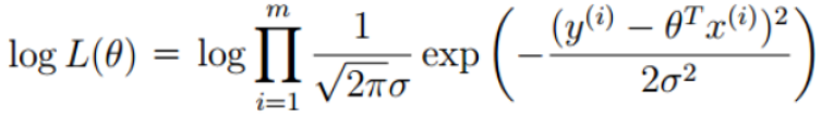
因为每个预测值都是独立分布的,所以我们要得到累乘概率(似然函数),但是由于计算原因,需要取对数(对数似然),如: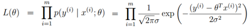
- 然后
化简得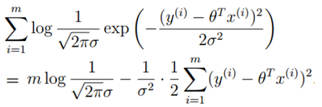 越大越好,即
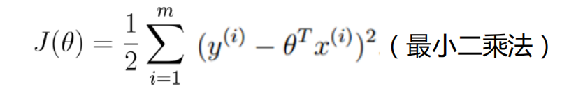 越小越好
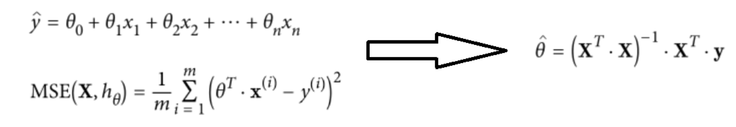
越小越好 - 然后求解θ(最小二乘法求解(矩阵可逆))
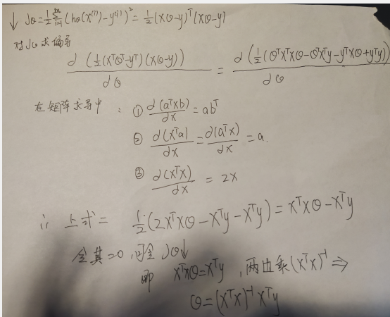
- 注意
此时逆不一定存在,而且还没有学习的过程,对于可以写出函数表达式的(可直接求解θ)可以直接用以上方法得到θ,但是大部分不使用该方法。使用梯度下降方法(常规套路)得到θ。
- 首先:
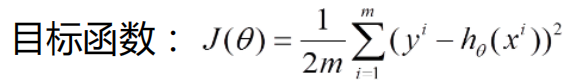
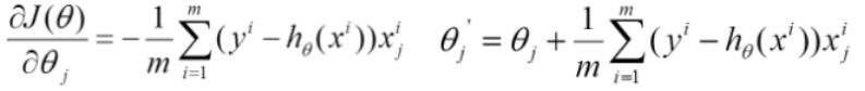
四.求解θ套路(梯度下降)
-
目标函数:

-
方法:
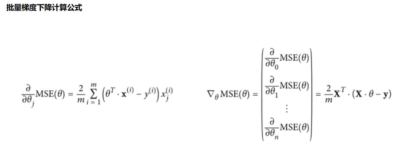
1.求方向
2.走小步
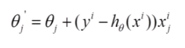
3.迭代更新参数 -
具体操作:
* 1.批量梯度法(需要数据量最多,但可以得到最优解)注意:m:越大越好,为什么平方:因为将原本差异变大,求偏导θj后可以得到一个方向,然后(-)反方向+θj开始走一小步,寻找最低点
* 2.随机梯度法 随机找一个数据(得到的不够准确,但是快)
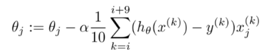
* 3.小梯度批量下降法(常用) 找部分数据,α为学习率:越小越好,为走小步的意思
五.代码实现
-
求θ原理
-
方法1:最下二乘法计算θ -
1.准备随机数据,并使用plt画出观察
import matplotlib import matplotlib.pyplot as plt import numpy as np #字体大小 plt.rcParams['axes.labelsize'] = 14 plt.rcParams['xtick.labelsize'] = 12 plt.rcParams['ytick.labelsize'] = 12 # 生成矩阵取值(0-2) 100个数 X = 2*np.random.rand(100,1) print(X) y = 4+ 3*X +np.random.randn(100,1) # b颜色,.是线条样式为. plt.plot(X,y,'b.') plt.title("数据") plt.xlabel('X_1') plt.ylabel('y') #x:取值0到2,y:取值0到15 plt.axis([0,2,0,15]) plt.show()
- 2.先对数据处理,增加一列x0为1,原因:三中已经介绍;再使用上述求解θ公式得到θ(矩阵)
X_b = np.c_[np.ones((100,1)),X] theta_best = np.linalg.inv(X_b.T.dot(X_b)).dot(X_b.T).dot(y) theta_best
- 3.构建测试数据矩阵,使用θ预测y,并画图对比
#预测 X_new = np.array([[0],[2]]) X_new_b = np.c_[np.ones((2,1)),X_new] y_predict = X_new_b.dot(theta_best) y_predict #画图 plt.plot(X_new,y_predict,'r--') plt.plot(X,y,'b.') plt.axis([0,2,0,15]) plt.show()
-
方法2:使用sklearn工具包中LinearRegression模型计算θ - 使用sklearn进行机器学习求解求θ原理 sklearn api文档
- 1.使用sklearn中模型求解θ
#导入工具包中线性回归模型 from sklearn.linear_model import LinearRegression #实例化 lin_reg = LinearRegression() lin_reg.fit(X,y) #权重参数 print (lin_reg.coef_) #偏置参数 print (lin_reg.intercept_)
-
方法3:使用批量梯度下降计算θ -
1.注意:步长过大或者过小问题(尽量调小),全局最下和局部最下问题(多做对比试验,学习率调小,初始化位置选择),进行标准化(减小数值浮动)
-
2.根据公式求解θ
#学习率:0.1,迭代次数:1000,样本个数:100,权重θ:theta为初始化随机(有两个),求和操作相当与矩阵操作 eta = 0.1 n_iterations = 1000 m = 100 theta = np.random.randn(2,1) for iteration in range(n_iterations): gradients = 2/m* X_b.T.dot(X_b.dot(theta)-y) theta = theta - eta*gradients theta
- 3.根据θ进行预测
y_predict2=X_new_b.dot(theta) y_predict2
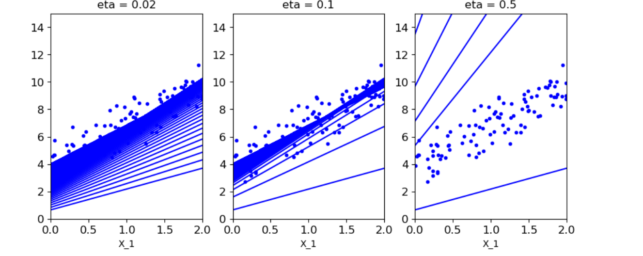
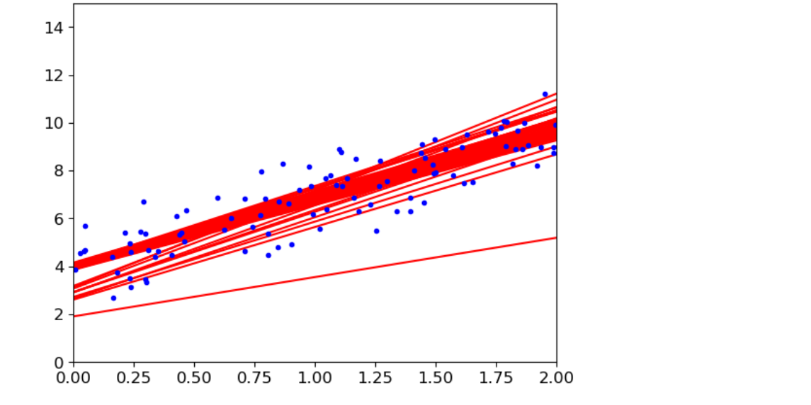
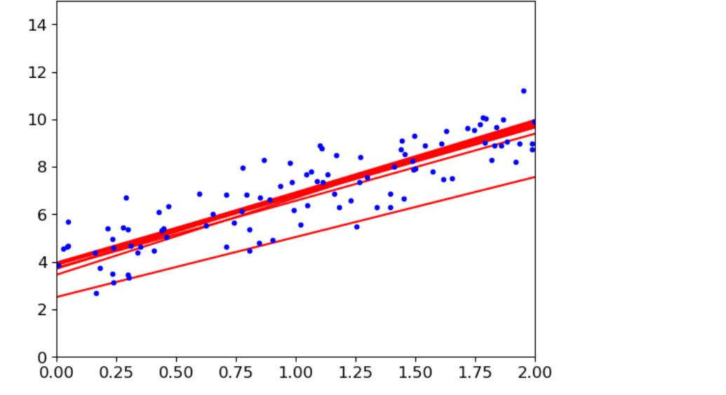
- 4.当学习率不同是,对结果的影响(得到结果:学习率类似表示图中线段中间隔;当学习率较大是,幅度过大,会越过最佳θ;当学习率较小,幅度较小,需要在递归很多次的时候θ才趋向稳定)
#1.theta_path_bgd用于存放不同策略的θ值 #2.n_iterations迭代次数 #3. plt.plot(X_new,y_predict,'b-')画出每一次迭代的预测值构成的直线 #4.if是去判断是否将θ存放到theta_path_bgd theta_path_bgd = [] def plot_gradient_descent(theta,eta,theta_path = None): m = len(X_b) plt.plot(X,y,'b.') n_iterations = 1000 for iteration in range(n_iterations): y_predict = X_new_b.dot(theta) plt.plot(X_new,y_predict,'b-') gradients = 2/m* X_b.T.dot(X_b.dot(theta)-y) theta = theta - eta*gradients if theta_path is not None: theta_path.append(theta) plt.xlabel('X_1') plt.axis([0,2,0,15]) plt.title('eta = {}'.format(eta)) theta = np.random.randn(2,1) #尺寸 plt.figure(figsize=(10,4)) #三个图第一个:学习率0.02 plt.subplot(131) plot_gradient_descent(theta,eta = 0.02) #三个图第二个:学习率0.1 plt.subplot(132) plot_gradient_descent(theta,eta = 0.1,theta_path=theta_path_bgd) #三个图第三个:学习率0.5 plt.subplot(133) plot_gradient_descent(theta,eta = 0.5) plt.show()
-
方法4:使用随机梯度下降计算θ
#取前几次画图 #theta_path_sgd保存随机策略的θ值 #n_epochs迭代次数50 #learning_schedule 学习率衰减策略(先全部(大),在局部(小)) #t迭代次数,随着迭代次数越大,学习率越小,越精细(t0,t1可随便取值) theta_path_sgd=[] m = len(X_b) np.random.seed(42) n_epochs = 50 t0 = 5 t1 = 50 def learning_schedule(t): return t0/(t1+t) theta = np.random.randn(2,1) #随机取得一个数,进行gradients求值从而结合衰减策略得到θ值,而后根据θ值求预测值并画图 for epoch in range(n_epochs): for i in range(m): random_index = np.random.randint(m) xi = X_b[random_index:random_index+1] yi = y[random_index:random_index+1] gradients = 2* xi.T.dot(xi.dot(theta)-yi) eta = learning_schedule(epoch*m+i) theta = theta-eta*gradients if epoch < 10 and i<10: y_predict = X_new_b.dot(theta) plt.plot(X_new,y_predict,'r-') theta_path_sgd.append(theta) plt.plot(X,y,'b.') plt.axis([0,2,0,15]) plt.show()
-
方法5:使用小梯度批量下降法计算θ
#theta_path_mgd保存小梯度批量下降策略的θ值 #对于迭代一次后,有个洗牌操作,X_b_shuffled是洗牌后新的迭代数据 #(0,m,minibatch)表示从第0个开始,到m结束,每次minibatch个 (找部分数据16个进行求解进行gradients求值从而结合衰减策略得到θ值,而后根据θ值求预测值并画图) theta_path_mgd=[] n_epochs = 50 minibatch = 16 theta = np.random.randn(2,1) t0, t1 = 200, 1000 def learning_schedule(t): return t0 / (t + t1) np.random.seed(42) t = 0 for epoch in range(n_epochs): shuffled_indices = np.random.permutation(m) X_b_shuffled = X_b[shuffled_indices] y_shuffled = y[shuffled_indices] for i in range(0,m,minibatch): t+=1 xi = X_b_shuffled[i:i+minibatch] yi = y_shuffled[i:i+minibatch] gradients = 2/minibatch* xi.T.dot(xi.dot(theta)-yi) eta = learning_schedule(t) theta = theta-eta*gradients if epoch < 10 and i<10: y_predict = X_new_b.dot(theta) plt.plot(X_new,y_predict,'r-') theta_path_mgd.append(theta) plt.plot(X,y,'b.') plt.axis([0,2,0,15]) plt.show()
-
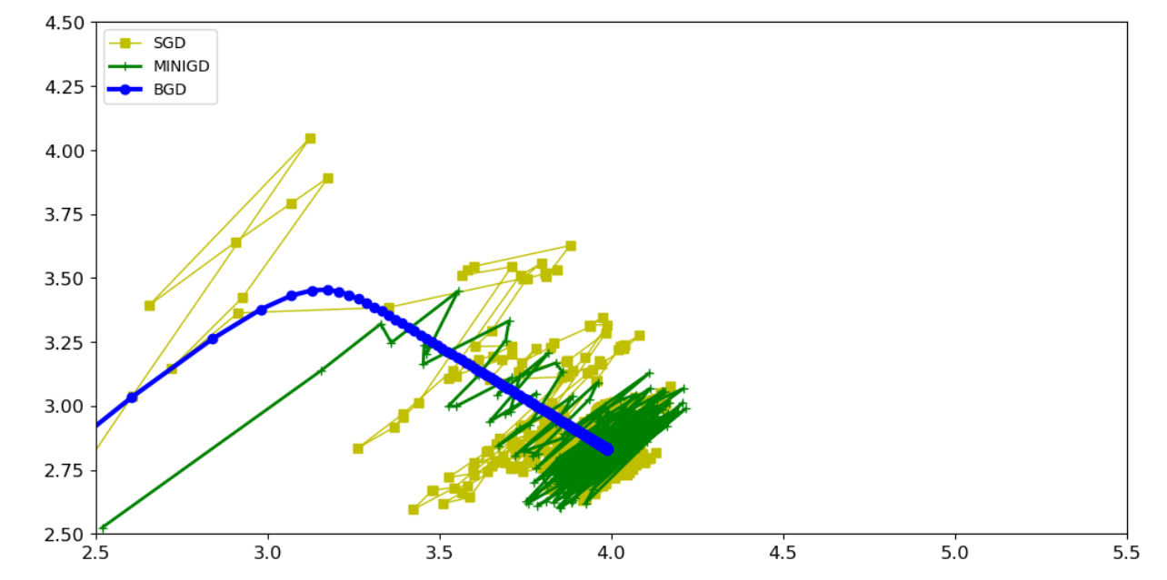
对比试验:方法3,方法4,方法5,结论:大部分试验使用方法5最多
# 将list转换为ndarray类型 theta_path_bgd = np.array(theta_path_bgd) theta_path_sgd = np.array(theta_path_sgd) theta_path_mgd = np.array(theta_path_mgd) type(theta_path_bgd) #展示 [:,0] 权重θ0和 [:,1] 偏置项θ1 plt.figure(figsize=(12,6)) plt.plot(theta_path_sgd[:,0],theta_path_sgd[:,1],'y-s',linewidth=1,label='SGD') plt.plot(theta_path_mgd[:,0],theta_path_mgd[:,1],'g-+',linewidth=2,label='MINIGD') plt.plot(theta_path_bgd[:,0],theta_path_bgd[:,1],'b-o',linewidth=3,label='BGD') plt.legend(loc='upper left') plt.axis([2.5,5.5,2.5,4.5]) plt.show()
六.多项式回归(y=x+x ²+b)
- 对二次,三次,多次等进行多项式回归预测
- 代码实现
- 对2次方,1次方组合预测
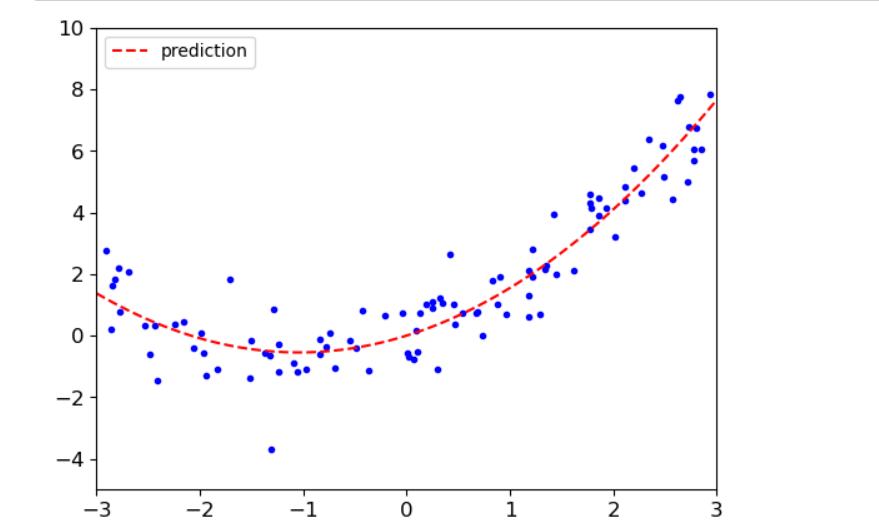
#对2次方,1次方组合预测 #m个点 #x取值-3到3 #np.random.randn(m,1)按正太分布的一个随机抖动 m = 100 X = 6*np.random.rand(m,1) - 3 y = 0.5*X**2+X+np.random.randn(m,1) #画散点图 #x取值范围-3到3,y取值范围-5到10 plt.plot(X,y,'b.') plt.xlabel('X_1') plt.ylabel('y') plt.axis([-3,3,-5,10]) plt.show() #使用sklearn中PolynomialFeatures将计算 x² from sklearn.preprocessing import PolynomialFeatures #实例化,include_bias = False是先不设置偏置项,得到[x,x²] poly_features = PolynomialFeatures(degree = 2,include_bias = False) #fit是训练得到结果,transform是将结果返回给Xpoly X_poly = poly_features.fit_transform(X) prinnt(X[0]) print(X_poly[0]) print(1.76886782 ** 2) #导入工具包中线性回归模型 #使用模型训练数据得到权重,生成y=1.046x+0.501x²-0.0004,得到多项式回归方程 from sklearn.linear_model import LinearRegression lin_reg = LinearRegression() lin_reg.fit(X_poly,y) print (lin_reg.coef_) print (lin_reg.intercept_) #生成数组-3到3,100个数,100行,1列 #使用transform,而不使用fit_transform是因为前面已经知道规则了,直接转换就行了。 #生成[x,x²] #使用模型预测y #画图 X_new = np.linspace(-3,3,100).reshape(100,1) X_new_poly = poly_features.transform(X_new) y_new = lin_reg.predict(X_new_poly) plt.plot(X,y,'b.') plt.plot(X_new,y_new,'r--',label='prediction') plt.axis([-3,3,-5,10]) #显示左上角标签 plt.legend(loc='upper left') plt.show()
- 对100次方,3次方,1次方多项式预测
#100次方,3次方,1次方多项式预测 #特征变换 #标准化 #训练模型 from sklearn.pipeline import Pipeline from sklearn.preprocessing import StandardScaler plt.figure(figsize=(12,6)) for style,width,degree in (('g-',1,100),('b--',2,3),('r-+',3,1)): #实例化特征变换,标准化,线性模型 poly_features = PolynomialFeatures(degree = degree,include_bias = False) std = StandardScaler() lin_reg = LinearRegression() #定义流水线车间的执行顺序 polynomial_reg = Pipeline([('poly_features',poly_features), ('StandardScaler',std), ('lin_reg',lin_reg)]) polynomial_reg.fit(X,y) #得到预测,然后画图 y_new_2 = polynomial_reg.predict(X_new) plt.plot(X_new,y_new_2,style,label = 'degree '+str(degree),linewidth = width) plt.plot(X,y,'b.') plt.axis([-3,3,-5,10]) plt.legend() plt.show()
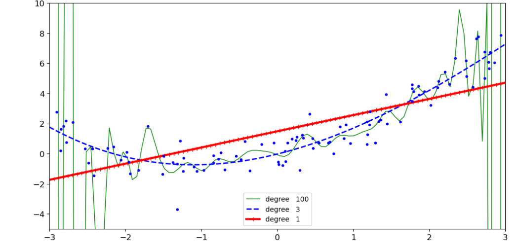
- 特征变换的越复杂,得到的结果过拟合风险越高,并且数据样本对过拟合影响也大。
- 样本数量产生过拟合对结果影响代码实现(线性回归,多项式回归)
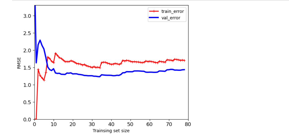
- 线性回归中样本数量对结果影响
#数据样本数量对过拟合的影响 #sklearn中的评估模块metrics,mean_squared_error均方误差 #random_state随机种子,可以使得运行任何一次得到的随机结果相同,即切分数据集模式不变 #X_train,y_tain训练集(80%),X_val,y_val验证集(20%) from sklearn.metrics import mean_squared_error from sklearn.model_selection import train_test_split def plot_learning_curves(model,X,y): X_train, X_val, y_train, y_val = train_test_split(X,y,test_size = 0.2,random_state=100) #train_errors 训练集的均方误差,val_errors 验证集的均方误差 train_errors,val_errors = [],[] #观察样本从一个到所有,误差变化情况 for m in range(1,len(X_train)): model.fit(X_train[:m],y_train[:m]) #训练集预测 y_train_predict = model.predict(X_train[:m]) #验证集预测 y_val_predict = model.predict(X_val) train_errors.append(mean_squared_error(y_train[:m],y_train_predict[:m])) val_errors.append(mean_squared_error(y_val,y_val_predict)) plt.plot(np.sqrt(train_errors),'r-+',linewidth = 2,label = 'train_error') plt.plot(np.sqrt(val_errors),'b-',linewidth = 3,label = 'val_error') plt.xlabel('Trainsing set size') plt.ylabel('RMSE') plt.legend() lin_reg = LinearRegression() plot_learning_curves(lin_reg,X,y) plt.axis([0,80,0,3.3]) plt.show()
- 多项式回归中样本数量对结果影响
#degree值越高,过拟合风险越大 polynomial_reg = Pipeline([('poly_features',PolynomialFeatures(degree = 25,include_bias = False)), ('lin_reg',LinearRegression())]) plot_learning_curves(polynomial_reg,X,y) plt.axis([0,80,0,5]) plt.show()
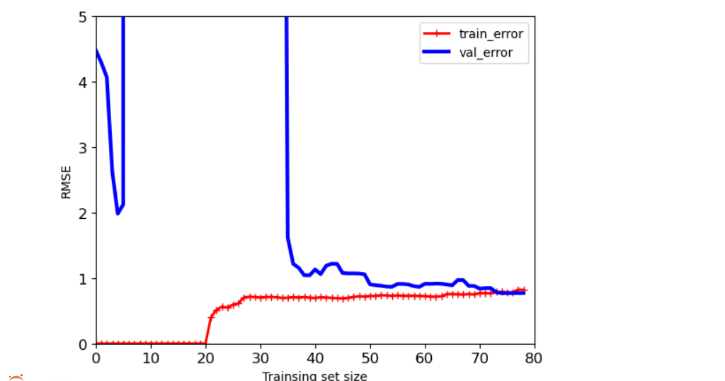
- 总结1:在[0,5]区间,训练集误差较小,但是实际验证时,却误差较大,出现过拟合;当数据量在[10,80],两条曲线是越来越接近的,误差比较稳定,过拟合风险较低。
- 总结1:数据量越少,训练集的效果会越好,但是实际测试效果很一般。实际做模型的时候需要参考测试集和验证集的效果。
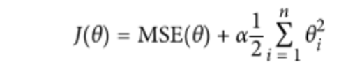
- 解决过拟合方法正则化
- 正则化 :对权重参数进行惩罚,α为惩罚项,越大说明后面比重越大,惩罚力度越大。让权重参数尽可能平滑一些,有两种不同的方法来进行正则化惩罚:岭回归(平方),lasso(绝对值)
MSE 均方误差 - 岭回归(平方)代码实现
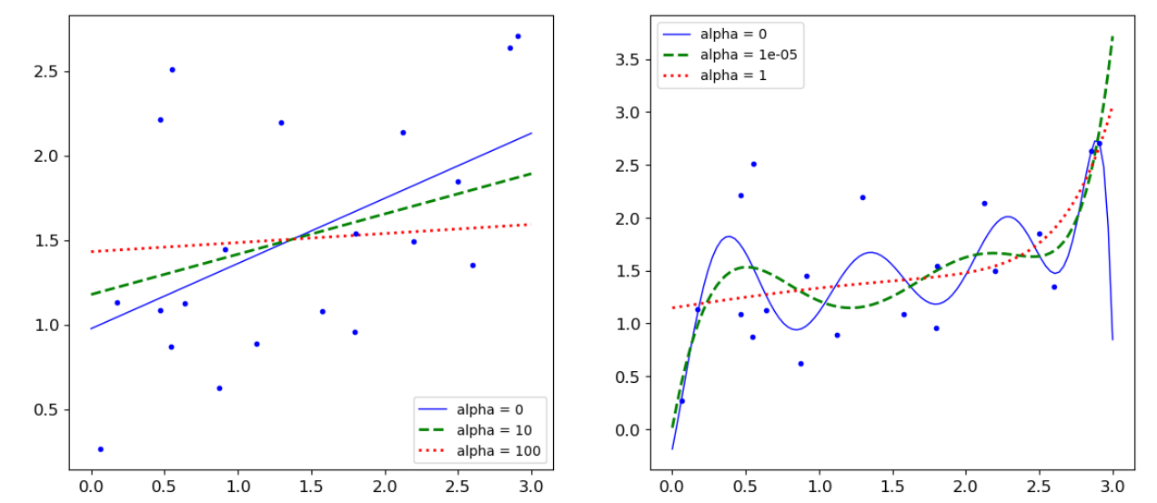
from sklearn.linear_model import Ridge np.random.seed(42) m = 20 X = 3*np.random.rand(m,1) y = 0.5 * X +np.random.randn(m,1)/1.5 +1 X_new = np.linspace(0,3,100).reshape(100,1) def plot_model(model_calss,polynomial,alphas,**model_kargs): #竖着对应如:alpha1对于b-,alpha2对应g--,alpha3对应r: for alpha,style in zip(alphas,('b-','g--','r:')): model = model_calss(alpha,**model_kargs) if polynomial: model = Pipeline([('poly_features',PolynomialFeatures(degree =10,include_bias = False)), ('StandardScaler',StandardScaler()), ('lin_reg',model)]) model.fit(X,y) y_new_regul = model.predict(X_new) #定义线条宽度 lw = 2 if alpha > 0 else 1 plt.plot(X_new,y_new_regul,style,linewidth = lw,label = 'alpha = {}'.format(alpha)) plt.plot(X,y,'b.',linewidth =3) plt.legend() plt.figure(figsize=(14,6)) #不加polynomial(多少次方degree) plt.subplot(121) plot_model(Ridge,polynomial=False,alphas = (0,10,100)) #加入polynomial(次方degree) plt.subplot(122) plot_model(Ridge,polynomial=True,alphas = (0,10**-5,1)) plt.show()
-
岭回归总结:对于第二个子图:当惩罚项较大时,决策方程越趋向于平稳
-
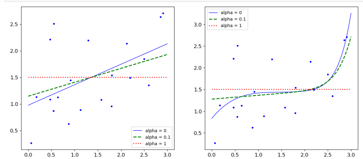
lasso(绝对值)代码实现

from sklearn.linear_model import Lasso plt.figure(figsize=(14,6)) plt.subplot(121) plot_model(Lasso,polynomial=False,alphas = (0,0.1,1)) plt.subplot(122) plot_model(Lasso,polynomial=True,alphas = (0,10**-1,1)) plt.show()


【推荐】国内首个AI IDE,深度理解中文开发场景,立即下载体验Trae
【推荐】编程新体验,更懂你的AI,立即体验豆包MarsCode编程助手
【推荐】抖音旗下AI助手豆包,你的智能百科全书,全免费不限次数
【推荐】轻量又高性能的 SSH 工具 IShell:AI 加持,快人一步
· 周边上新:园子的第一款马克杯温暖上架
· 分享 3 个 .NET 开源的文件压缩处理库,助力快速实现文件压缩解压功能!
· Ollama——大语言模型本地部署的极速利器
· DeepSeek如何颠覆传统软件测试?测试工程师会被淘汰吗?
· 使用C#创建一个MCP客户端