OpenCV实战（4）——文档扫描OCR识别&答题卡识别判卷（文档扫描，图像矫正，透视变换，OCR识别）

如果需要处理的原图及代码，请移步小编的GitHub地址

　　传送门：请点击我

　　如果点击有误：https://github.com/LeBron-Jian/ComputerVisionPractice

　　下面准备学习如何对文档扫描摆正及其OCR识别的案例，主要想法是对一张不规则的文档进行矫正，然后通过tesseract进行OCR文字识别，最后返回结果。下面进入正文：

　　现代生活中，手机像素比较高，所以大家拍这些照片都很随意，随便拍，比如下面的照片，如发票，文本等等：

　　对于这些图像矫正的问题，在图像处理领域还真的很多，比如文本的矫正，车牌的矫正，身份证的矫正等等。这些都是因为拍摄者拍照随意，这就要求我们通过后期的图像处理技术将图片还原好，才能进行下一步处理，比如数字分割，数字识别，字母识别，文字识别等等。

　　上面的问题，我们在日常生活中遇到的可不少，因为拍摄时拍的不好，导致拍出来的图片歪歪扭扭的，很不自然，那么我们如何将图片矫正过来呢？

　　总的来说，要进行图像矫正，至少需要以下几步：

1，文档的轮廓提取技术
2，原始与变换坐标的计算
3，通过透视变换获取目标区域

　　本文通过两个案例，一个是菜单矫正及OCR识别；另一个是答题卡矫正及OCR识别。

项目实战1——文档扫描OCR识别

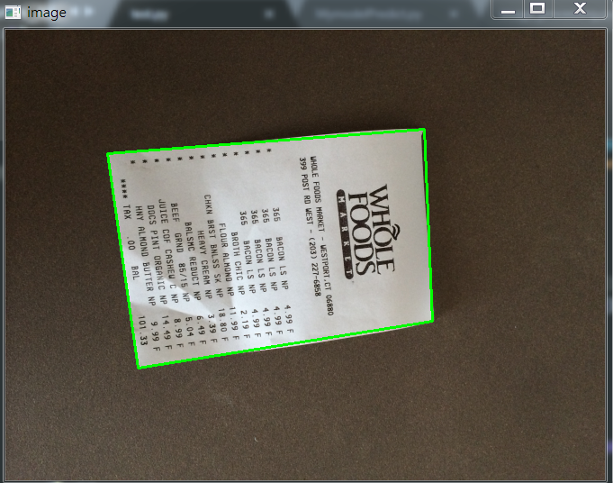
　　下面以菜单为例，慢慢剖析如何实现图像矫正，并获取菜单内容。

　　上面的斜着的菜单，如何扫描到如右图所示的照片呢？其实步骤有以下几步：

1，探测边缘
2，提取菜单矩阵轮廓四点进行透视变换
3，应用一个透视的转换去获取一个文档的自顶向下的正图

　　知道步骤后，我们开始做吧！

1.1，文档轮廓提取

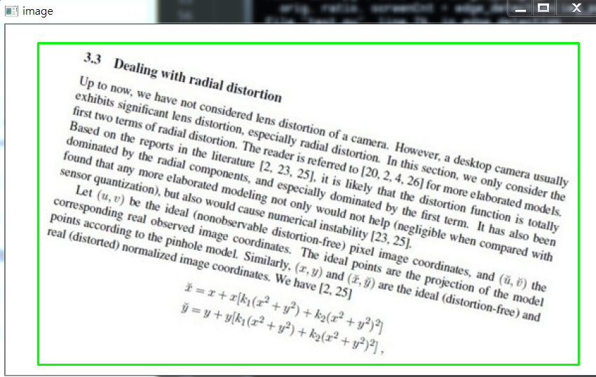
　　我们拿到图像之后，首先进行边缘检测，其中预处理包括对噪音进行高斯模糊，然后进行边缘检测（这里采用了Canny算子提取特征），下面我们可以看一下边缘检测的代码与结果：

　　代码：

def edge_detection(img_path):
    # 读取输入
    img = cv2.imread(img_path)
    # 坐标也会相同变换
    ratio = img.shape[0] / 500.0
    orig = img.copy()
 
    image = resize(orig, height=500)
    # 预处理
    gray = cv2.cvtColor(image, cv2.COLOR_BGR2GRAY)
    blur = cv2.GaussianBlur(gray, (5, 5), 0)
    edged = cv2.Canny(blur, 75, 200)
    show(edged)

　　效果如下：

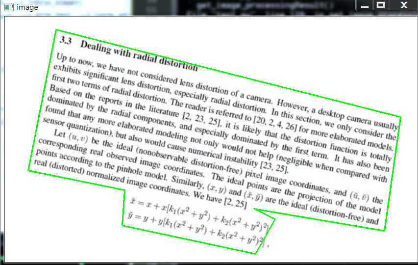
　　我们从上图可以看到，已经将菜单的所有轮廓都检测出来了，而我们其实只需要最外面的轮廓，下面我们通过过滤得到最边缘的轮廓即可。

　　代码如下：

def edge_detection(img_path):
    # *********  预处理 ****************
    # 读取输入
    img = cv2.imread(img_path)
    # 坐标也会相同变换
    ratio = img.shape[0] / 500.0
    orig = img.copy()
 
    image = resize(orig, height=500)
    # 预处理
    gray = cv2.cvtColor(image, cv2.COLOR_BGR2GRAY)
    blur = cv2.GaussianBlur(gray, (5, 5), 0)
    edged = cv2.Canny(blur, 75, 200)
 
    # *************  轮廓检测 ****************
    # 轮廓检测
    contours, hierarchy = cv2.findContours(edged.copy(), cv2.RETR_LIST, cv2.CHAIN_APPROX_SIMPLE)
    cnts = sorted(contours, key=cv2.contourArea, reverse=True)[:5]
 
    # 遍历轮廓
    for c in cnts:
        # 计算轮廓近似
        peri = cv2.arcLength(c, True)
        # c表示输入的点集，epsilon表示从原始轮廓到近似轮廓的最大距离，它是一个准确度参数
        approx = cv2.approxPolyDP(c, 0.02*peri, True)
 
        # 4个点的时候就拿出来
        if len(approx) == 4:
            screenCnt = approx
            break
 
    res = cv2.drawContours(image, [screenCnt], -1, (0, 255, 0), 2)
    show(res)

　　效果如下：

　　如果说对轮廓排序后，不进行近似的话，我们直接取最大的轮廓，效果图如下：

1.2，透视变换（摆正图像）

　　当获取到图片的最外轮廓后，接下来，我们需要摆正图像，在摆正图形之前，我们需要先学习透视变换。

1.2.1，cv2.getPerspectiveTransform()

　　透视变换（Perspective Transformation）是将成像投影到一个新的视平面（Viewing Plane），也称作投影映射（Projective mapping），如下图所示，通过透视变换ABC变换到A'B'C'。

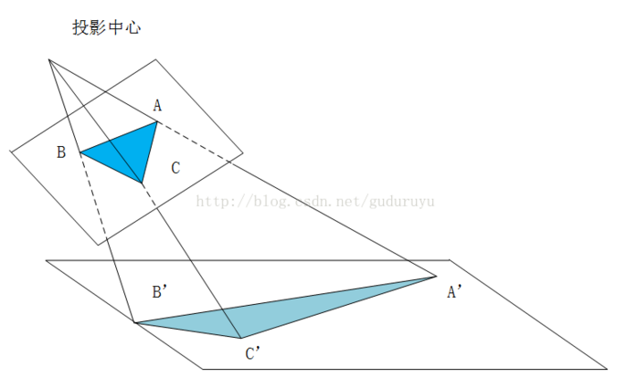
　　cv2.getPerspectiveTransform() 获取投射变换后的H矩阵。

　　cv2.getPerspectiveTransform() 函数的opencv 源码如下：

def getPerspectiveTransform(src, dst, solveMethod=None): # real signature unknown; restored from __doc__
    """
    getPerspectiveTransform(src, dst[, solveMethod]) -> retval
    .   @brief Calculates a perspective transform from four pairs of the corresponding points.
    .   
    .   The function calculates the \f$3 \times 3\f$ matrix of a perspective transform so that:
    .   
    .   \f[\begin{bmatrix} t_i x'_i \\ t_i y'_i \\ t_i \end{bmatrix} = \texttt{map_matrix} \cdot \begin{bmatrix} x_i \\ y_i \\ 1 \end{bmatrix}\f]
    .   
    .   where
    .   
    .   \f[dst(i)=(x'_i,y'_i), src(i)=(x_i, y_i), i=0,1,2,3\f]
    .   
    .   @param src Coordinates of quadrangle vertices in the source image.
    .   @param dst Coordinates of the corresponding quadrangle vertices in the destination image.
    .   @param solveMethod method passed to cv::solve (#DecompTypes)
    .   
    .   @sa  findHomography, warpPerspective, perspectiveTransform
    """
    pass

　　参数说明：

rect（即函数中src）表示待测矩阵的左上，右上，右下，左下四点坐标
transform_axes（即函数中dst）表示变换后四个角的坐标，即目标图像中矩阵的坐标

　　返回值由原图像中矩阵到目标图像矩阵变换的矩阵，得到矩阵接下来则通过矩阵来获得变换后的图像，下面我们学习第二个函数。

1.2.2，cv2.warpPerspective()

　　cv2.warpPerspective() 根据H获得变换后的图像。

　　opencv源码如下：

def warpPerspective(src, M, dsize, dst=None, flags=None, borderMode=None, borderValue=None): # real signature unknown; restored from __doc__
    """
    warpPerspective(src, M, dsize[, dst[, flags[, borderMode[, borderValue]]]]) -> dst
    .   @brief Applies a perspective transformation to an image.
    .   
    .   The function warpPerspective transforms the source image using the specified matrix:
    .   
    .   \f[\texttt{dst} (x,y) =  \texttt{src} \left ( \frac{M_{11} x + M_{12} y + M_{13}}{M_{31} x + M_{32} y + M_{33}} ,
    .        \frac{M_{21} x + M_{22} y + M_{23}}{M_{31} x + M_{32} y + M_{33}} \right )\f]
    .   
    .   when the flag #WARP_INVERSE_MAP is set. Otherwise, the transformation is first inverted with invert
    .   and then put in the formula above instead of M. The function cannot operate in-place.
    .   
    .   @param src input image.
    .   @param dst output image that has the size dsize and the same type as src .
    .   @param M \f$3\times 3\f$ transformation matrix.
    .   @param dsize size of the output image.
    .   @param flags combination of interpolation methods (#INTER_LINEAR or #INTER_NEAREST) and the
    .   optional flag #WARP_INVERSE_MAP, that sets M as the inverse transformation (
    .   \f$\texttt{dst}\rightarrow\texttt{src}\f$ ).
    .   @param borderMode pixel extrapolation method (#BORDER_CONSTANT or #BORDER_REPLICATE).
    .   @param borderValue value used in case of a constant border; by default, it equals 0.
    .   
    .   @sa  warpAffine, resize, remap, getRectSubPix, perspectiveTransform
    """
    pass

　　参数说明：

src 表示输入的灰度图像
M 表示变换矩阵
dsize 表示目标图像的shape，（width, height）表示变换后的图像大小
flags：插值方式，interpolation方法INTER_LINEAR或者INTER_NEAREST
borderMode：边界补偿方式，BORDER_CONSTANT or BORDER_REPLCATE
borderValue：边界补偿大小，常值，默认为0

1.2.3 cv2.perspectiveTransform()

　　cv2.perspectiveTransform() 和 cv2.warpPerspective()大致作用相同，但是区别在于 cv2.warpPerspective()适用于图像，而cv2.perspectiveTransform() 适用于一组点。

　　cv2.perspectiveTransform() 的opencv源码如下：

def perspectiveTransform(src, m, dst=None): # real signature unknown; restored from __doc__
    """
    perspectiveTransform(src, m[, dst]) -> dst
    .   @brief Performs the perspective matrix transformation of vectors.
    .   
    .   The function cv::perspectiveTransform transforms every element of src by
    .   treating it as a 2D or 3D vector, in the following way:
    .   \f[(x, y, z)  \rightarrow (x'/w, y'/w, z'/w)\f]
    .   where
    .   \f[(x', y', z', w') =  \texttt{mat} \cdot \begin{bmatrix} x & y & z & 1  \end{bmatrix}\f]
    .   and
    .   \f[w =  \fork{w'}{if \(w' \ne 0\)}{\infty}{otherwise}\f]
    .   
    .   Here a 3D vector transformation is shown. In case of a 2D vector
    .   transformation, the z component is omitted.
    .   
    .   @note The function transforms a sparse set of 2D or 3D vectors. If you
    .   want to transform an image using perspective transformation, use
    .   warpPerspective . If you have an inverse problem, that is, you want to
    .   compute the most probable perspective transformation out of several
    .   pairs of corresponding points, you can use getPerspectiveTransform or
    .   findHomography .
    .   @param src input two-channel or three-channel floating-point array; each
    .   element is a 2D/3D vector to be transformed.
    .   @param dst output array of the same size and type as src.
    .   @param m 3x3 or 4x4 floating-point transformation matrix.
    .   @sa  transform, warpPerspective, getPerspectiveTransform, findHomography
    """
    pass

　　参数含义：

src：输入的二通道或三通道的图像
m：变换矩阵
返回结果为相同size的图像

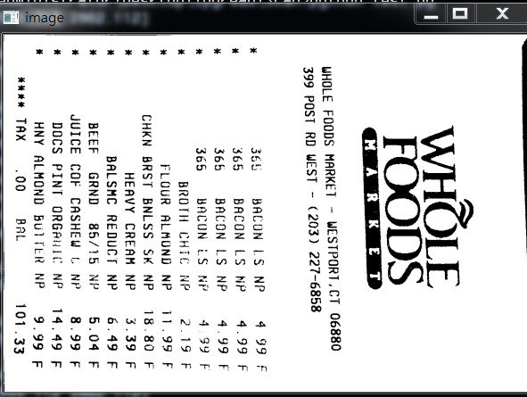
1.2.4 摆正图像

　　将图像框出来后，我们计算出变换前后的四个点的坐标，然后得到最终的变换结果。

　　代码如下：

def order_points(pts):
    # 一共四个坐标点
    rect = np.zeros((4, 2), dtype='float32')
     
    # 按顺序找到对应的坐标0123 分别是左上，右上，右下，左下
    # 计算左上，由下
    # numpy.argmax(array, axis) 用于返回一个numpy数组中最大值的索引值
    s = pts.sum(axis=1)  # [2815.2   1224.    2555.712 3902.112]
    print(s)
    rect[0] = pts[np.argmin(s)]
    rect[2] = pts[np.argmax(s)]
 
    # 计算右上和左
    # np.diff()  沿着指定轴计算第N维的离散差值  后者-前者
    diff = np.diff(pts, axis=1)
    rect[1] = pts[np.argmin(diff)]
    rect[3] = pts[np.argmax(diff)]
    return rect
 
 
# 透视变换
def four_point_transform(image, pts):
    # 获取输入坐标点
    rect = order_points(pts)
    (tl, tr, br, bl) = rect
 
    # 计算输入的w和h的值
    widthA = np.sqrt(((br[0] - bl[0])**2) + ((br[1] - bl[1])**2))
    widthB = np.sqrt(((tr[0] - tl[0])**2) + ((tr[1] - tl[1])**2))
    maxWidth = max(int(widthA), int(widthB))
 
    heightA = np.sqrt(((tr[0] - br[0])**2) + ((tr[1] - br[1])**2))
    heightB = np.sqrt(((tl[0] - bl[0])**2) + ((tl[1] - bl[1])**2))
    maxHeight = max(int(heightA), int(heightB))
 
    # 变化后对应坐标位置
    dst = np.array([
        [0, 0],
        [maxWidth - 1, 0],
        [maxWidth - 1, maxHeight - 1],
        [0, maxHeight - 1]],
        dtype='float32')    
 
    # 计算变换矩阵
    M = cv2.getPerspectiveTransform(rect, dst)
    warped = cv2.warpPerspective(image, M, (maxWidth, maxHeight))
 
    # 返回变换后的结果
    return warped
 
 
# 对透视变换结果进行处理
def get_image_processingResult():
    img_path = 'images/receipt.jpg'
    orig, ratio, screenCnt = edge_detection(img_path)
    # screenCnt 为四个顶点的坐标值，但是我们这里需要将图像还原，即乘以以前的比率
    # 透视变换  这里我们需要将变换后的点还原到原始坐标里面
    warped = four_point_transform(orig, screenCnt.reshape(4, 2)*ratio)
    # 二值处理
    gray = cv2.cvtColor(warped, cv2.COLOR_BGR2GRAY)
    thresh = cv2.threshold(gray, 100, 255, cv2.THRESH_BINARY)[1]
 
    thresh_resize = resize(thresh, height = 400)
    show(thresh_resize)

　　效果如下：

1.2.5 其他图片矫正实践

　　这里图片原图都可以去我的GitHub里面去拿（地址：https://github.com/LeBron-Jian/ComputerVisionPractice）。

　　对于下面这张图：

　　我们使用透视变换抠出来效果如下：

　　这个图使用和之前的代码就可以，不用修改任何东西就可以拿到其目标区域。

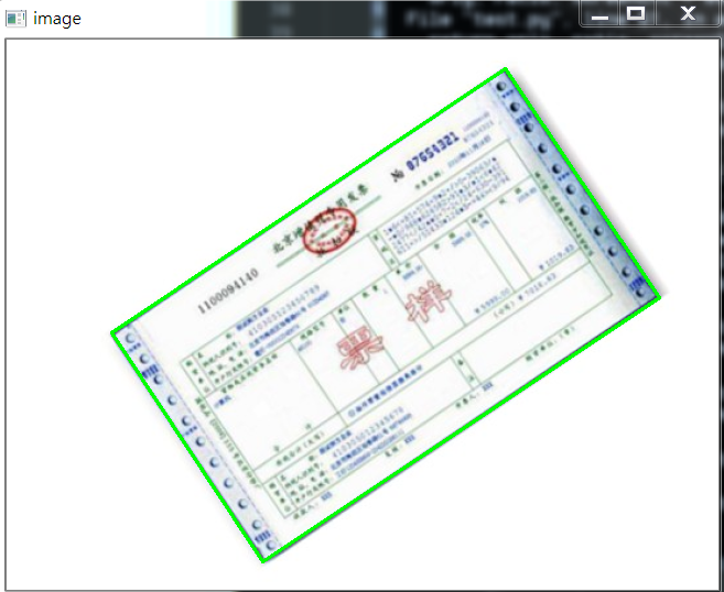
　　下面看这张图：

　　其实和上面图类似，不过这里我们依次看一下其图像处理过程，毕竟和上面两张图完全不是一个类型了。

　　首先是 Canny算子得到的结果：

　　其实拿到全轮廓后，我们就直接获取最外面的轮廓即可。

　　我自己更改了一下，效果一样，但是还是贴上代码：

def edge_detection(img_path):
    # *********  预处理 ****************
    # 读取输入
    img = cv2.imread(img_path)
    # 坐标也会相同变换
    ratio = img.shape[0] / 500.0
    orig = img.copy()
 
    image = resize(orig, height=500)
    # 预处理
    gray = cv2.cvtColor(image, cv2.COLOR_BGR2GRAY)
    blur = cv2.GaussianBlur(gray, (5, 5), 0)
    edged = cv2.Canny(blur, 75, 200)
    # show(edged)
    # *************  轮廓检测 ****************
    # 轮廓检测
    contours, hierarchy = cv2.findContours(edged.copy(), cv2.RETR_LIST, cv2.CHAIN_APPROX_SIMPLE)
    #cnts = sorted(contours, key=cv2.contourArea, reverse=True)[:5]
 
    max_area = 0
    myscreenCnt = []
    for i in contours:
        temp = cv2.contourArea(i)
        if max_area < temp:
            myscreenCnt = i
 
    # res = cv2.drawContours(image, myscreenCnt, -1, (0, 255, 0), 2)
    # show(res)
    return orig, ratio, screenCnt

　　最后我们不对发票做任何处理，看原图效果：

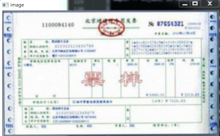
　　部分代码如下：

# 对透视变换结果进行处理
def get_image_processingResult():
    img_path = 'images/fapiao.jpg'
    orig, ratio, screenCnt = edge_detection(img_path)
    # screenCnt 为四个顶点的坐标值，但是我们这里需要将图像还原，即乘以以前的比率
    # 透视变换  这里我们需要将变换后的点还原到原始坐标里面
    warped = four_point_transform(orig, screenCnt.reshape(4, 2)*ratio)
 
    thresh_resize = resize(warped, height = 400)
    show(thresh_resize)
    return thresh

　　下面再看一个例子：

　　首先，它得到的Canny结果如下：

　　我们需要对它进行一些小小的处理。

　　我做了一些尝试，如果直接对膨胀后的图像，进行外接矩形，那么效果如下：

　　代码如下：

x, y, w, h = cv2.boundingRect(myscreenCnt)
res = cv2.rectangle(image, (x,y), (x+w,y+h), (0, 255, 0), 2)
show(res)

　　所以对轮廓取近似，效果稍微好点：

# 计算轮廓近似
peri = cv2.arcLength(myscreenCnt, True)
# c表示输入的点集，epsilon表示从原始轮廓到近似轮廓的最大距离，它是一个准确度参数
approx = cv2.approxPolyDP(myscreenCnt, 0.015*peri, True)
res = cv2.drawContours(image, [approx], -1, (0, 255, 0), 2)
show(res)

　　效果如下：

　　因为这个是不规整图形，所以无法进行四个角的转换，需要更多角，这里不再继续尝试。

1.3，OCR识别

　　这里回到我们的菜单来，我们已经得到了扫描后的结果，下面我们进行OCR文字识别。

　　这里使用tesseract进行识别，不懂的可以参考我之前的博客（包括安装tesseract，和通过tesseract训练自己的字库）：

深入学习使用ocr算法识别图片中文字的方法

深入学习Tesseract-ocr识别中文并训练字库的方法

　　配置好tesseract之后（这里不再show过程，因为我已经有了），我们通过其进行文字识别。

1.3.1 通过Python使用tesseract的坑

　　如果直接使用Python进行OCR识别的话，会出现下面问题：

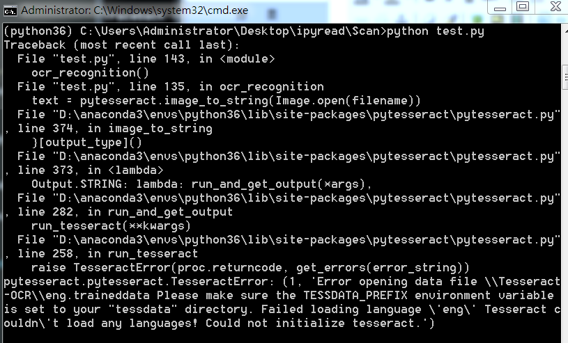
　　这里因为anaconda下载的 pytesseract 默认运行的tesseract.exe 是默认文件夹，所以有问题，我们改一下。

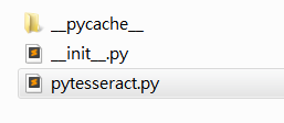
　　注意，找到安装地址，我们会发现有两个文件夹，我们进入上面文件夹即可

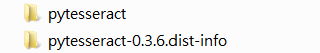
　　进入之后如下，我们打开 pytesseract.py。

　　注意这里的地址：

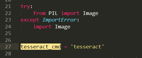
　　我们需要修改为我们安装的地址，即使我们之前设置了全局变量，但是Python还是不care的。

　　这里注意地址的话，我们通过 / 即可，不要 \，避免windows出现问题。

1.3.2 OCR识别

　　安装好一切之后，就可以识别了，我们这里有两种方法，一种是直接在人家的环境下运行，一种是在Python中通过安装pytesseract 库运行，效果都一样。

　　代码如下：

from PIL import Image
import pytesseract
import cv2
import os
 
preprocess = 'blur' #thresh
 
image = cv2.imread('scan.jpg')
gray = cv2.cvtColor(image, cv2.COLOR_BGR2GRAY)
 
if preprocess == "thresh":
    gray = cv2.threshold(gray, 0, 255,cv2.THRESH_BINARY | cv2.THRESH_OTSU)[1]
 
if preprocess == "blur":
    gray = cv2.medianBlur(gray, 3)
     
filename = "{}.png".format(os.getpid())
cv2.imwrite(filename, gray)
     
text = pytesseract.image_to_string(Image.open(filename))
print(text)
os.remove(filename)
 
cv2.imshow("Image", image)
cv2.imshow("Output", gray)
cv2.waitKey(0)                                   

　　使用Python运行，效果如下：

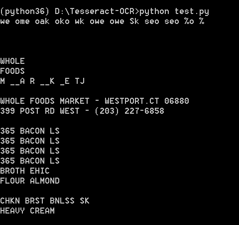
　　直接在tesseract.exe运行：

　　效果如下：

　　可能识别效果不是很好。不过不重要，因为图片也比较模糊，不是那么工整的。

1.4，完整代码

　　当然也可以去我的GitHub直接去下载。

　　代码如下：

100

101

102

103

104

105

106

107

108

109

110

111

112

113

114

115

116

117

118

119

120

121

122

123

124

125

126

127

128

129

130

131

132

133

134

135

136

137

138

139

140

141

142

143

144

import cv2
import numpy as np
from PIL import Image
import pytesseract
 
 
def show(image):
    cv2.imshow('image', image)
    cv2.waitKey(0)
    cv2.destroyAllWindows()
 
def resize(image, width=None, height=None, inter=cv2.INTER_AREA):
    dim = None
    (h, w) = image.shape[:2]
    if width is None and height is None:
        return image
    if width is None:
        r = height / float(h)
        dim = (int(w*r), height)
    else:
        r = width / float(w)
        dim = (width, int(h*r))
    resized = cv2.resize(image, dim, interpolation=inter)
    return resized
 
 
def edge_detection(img_path):
    # *********  预处理 ****************
    # 读取输入
    img = cv2.imread(img_path)
    # 坐标也会相同变换
    ratio = img.shape[0] / 500.0
    orig = img.copy()
 
    image = resize(orig, height=500)
    # 预处理
    gray = cv2.cvtColor(image, cv2.COLOR_BGR2GRAY)
    blur = cv2.GaussianBlur(gray, (5, 5), 0)
    edged = cv2.Canny(blur, 75, 200)
 
    # *************  轮廓检测 ****************
    # 轮廓检测
    contours, hierarchy = cv2.findContours(edged.copy(), cv2.RETR_LIST, cv2.CHAIN_APPROX_SIMPLE)
    cnts = sorted(contours, key=cv2.contourArea, reverse=True)[:5]
 
    # 遍历轮廓
    for c in cnts:
        # 计算轮廓近似
        peri = cv2.arcLength(c, True)
        # c表示输入的点集，epsilon表示从原始轮廓到近似轮廓的最大距离，它是一个准确度参数
        approx = cv2.approxPolyDP(c, 0.02*peri, True)
 
        # 4个点的时候就拿出来
        if len(approx) == 4:
            screenCnt = approx
            break
 
    # res = cv2.drawContours(image, [screenCnt], -1, (0, 255, 0), 2)
    # res = cv2.drawContours(image, cnts[0], -1, (0, 255, 0), 2)
    # show(orig)
    return orig, ratio, screenCnt
 
 
def order_points(pts):
    # 一共四个坐标点
    rect = np.zeros((4, 2), dtype='float32')
     
    # 按顺序找到对应的坐标0123 分别是左上，右上，右下，左下
    # 计算左上，由下
    # numpy.argmax(array, axis) 用于返回一个numpy数组中最大值的索引值
    s = pts.sum(axis=1)  # [2815.2   1224.    2555.712 3902.112]
    print(s)
    rect[0] = pts[np.argmin(s)]
    rect[2] = pts[np.argmax(s)]
 
    # 计算右上和左
    # np.diff()  沿着指定轴计算第N维的离散差值  后者-前者
    diff = np.diff(pts, axis=1)
    rect[1] = pts[np.argmin(diff)]
    rect[3] = pts[np.argmax(diff)]
    return rect
 
 
# 透视变换
def four_point_transform(image, pts):
    # 获取输入坐标点
    rect = order_points(pts)
    (tl, tr, br, bl) = rect
 
    # 计算输入的w和h的值
    widthA = np.sqrt(((br[0] - bl[0])**2) + ((br[1] - bl[1])**2))
    widthB = np.sqrt(((tr[0] - tl[0])**2) + ((tr[1] - tl[1])**2))
    maxWidth = max(int(widthA), int(widthB))
 
    heightA = np.sqrt(((tr[0] - br[0])**2) + ((tr[1] - br[1])**2))
    heightB = np.sqrt(((tl[0] - bl[0])**2) + ((tl[1] - bl[1])**2))
    maxHeight = max(int(heightA), int(heightB))
 
    # 变化后对应坐标位置
    dst = np.array([
        [0, 0],
        [maxWidth - 1, 0],
        [maxWidth - 1, maxHeight - 1],
        [0, maxHeight - 1]],
        dtype='float32')    
 
    # 计算变换矩阵
    M = cv2.getPerspectiveTransform(rect, dst)
    warped = cv2.warpPerspective(image, M, (maxWidth, maxHeight))
 
    # 返回变换后的结果
    return warped
 
 
# 对透视变换结果进行处理
def get_image_processingResult():
    img_path = 'images/receipt.jpg'
    orig, ratio, screenCnt = edge_detection(img_path)
    # screenCnt 为四个顶点的坐标值，但是我们这里需要将图像还原，即乘以以前的比率
    # 透视变换  这里我们需要将变换后的点还原到原始坐标里面
    warped = four_point_transform(orig, screenCnt.reshape(4, 2)*ratio)
    # 二值处理
    gray = cv2.cvtColor(warped, cv2.COLOR_BGR2GRAY)
    thresh = cv2.threshold(gray, 100, 255, cv2.THRESH_BINARY)[1]
 
    cv2.imwrite('scan.jpg', thresh)
 
    thresh_resize = resize(thresh, height = 400)
    # show(thresh_resize)
    return thresh
 
 
 
def ocr_recognition(filename='tes.jpg'):
    img = Image.open(filename)
    text = pytesseract.image_to_string(img)
    print(text)
 
 
if __name__ == '__main__':
    # 获取矫正之后的图片
    # get_image_processingResult()
    # 进行OCR文字识别
    ocr_recognition()

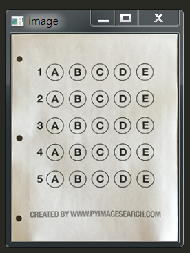
项目实战2——答题卡识别判卷

　　答题卡识别判卷，大家应该都不陌生。那么它需要做什么呢？肯定是将我们在答题卡上画圈圈的地方识别出来。

　　这是答题卡样子（原图请去我GitHub上拿：https://github.com/LeBron-Jian/ComputerVisionPractice）：

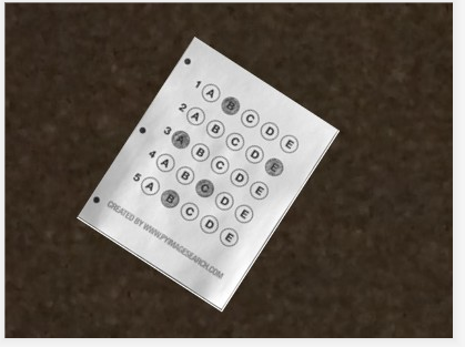
　　我们肯定是需要分为两步走，第一步就是和上面处理类似，拿到答题卡的最终透视变换结果，使得图片中的答题卡可以凸显出来。第二步就是根据正确答案和答题卡的答案来判断正确率。

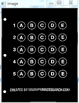
2.1 扫描答题卡及透视变换

　　这里我们对答题卡进行透视变换，因为之前已经详细的学习了这一部分，这里不再赘述，只是简单记录一下流程和图像处理效果，并展示代码。

　　下面详细的总结处理步骤：

1，图像灰度化
2，高斯滤波处理
3，使用Canny算子找到图片边缘信息
4，寻找轮廓
5，找到最外层轮廓，并确定四个坐标点
6，根据四个坐标位置计算出变换后的四个角位置
7，获取变换矩阵H，得到最终变换结果

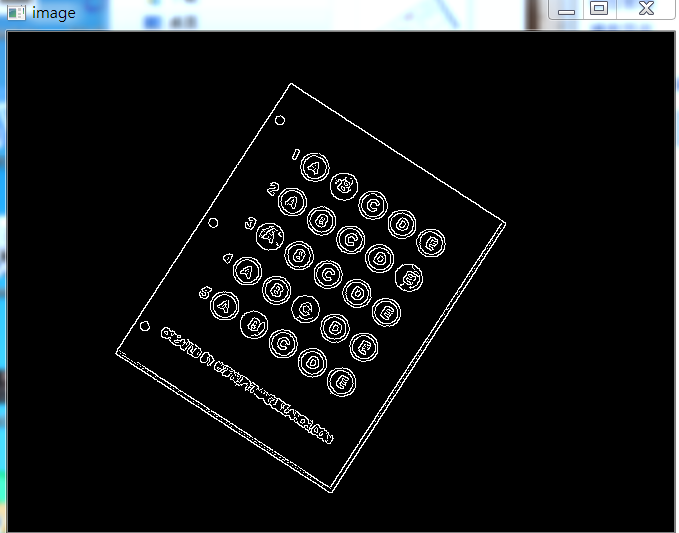
　　下面直接使用上面代码进行跑，首先展示Canny效果：

　　当Canny效果不错的时候，我们拿到图像的轮廓进行筛选，找到最外面的轮廓，如下图所示：

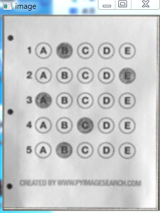
　　最后通过透视变换，获得答题卡的区域，如下图所示：

2.2 根据正确答案和图卡判断正确率

　　这里我们拿到上面得到的答题卡图像，然后进行操作，获取到涂的位置，然后和正确答案比较，最后获得正确率。

　　这里分为以下几个步骤：

1，对图像进行二值化，将涂了颜色的地方变为白色
2，对轮廓进行筛选，找到正确答案的轮廓
3，对轮廓从上到下进行排序
4，计算颜色最大值的位置和Nonezeros的值
5，结合正确答案计算正确率
6，将正确答案打印在图像上

　　下面开始实践：

　　首先对图像进行二值化，如下图所示：

　　如果对二值化后的图直接进行画轮廓，如下：

　　所以不能直接处理，这里我们需要做细微处理，然后拿到图像如下：

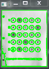
　　这样就可以获得其涂的轮廓，如下所示：

　　然后筛选出我们需要的涂了答题卡的位置，效果如下：

　　然后通过这五个坐标点，确定答题卡的位置，如下图所示：

　　然后根据真实答案和图中答案对比结果，我们将最终结果与圈出来答案展示在图上，如下：

　　此项目到此结束。

2.3 部分代码展示

　　完整代码可以去我的GitHub上拿（地址：https://github.com/LeBron-Jian/ComputerVisionPractice）

　　代码如下：

import cv2
import numpy as np
from PIL import Image
import pytesseract
 
 
def show(image):
    cv2.imshow('image', image)
    cv2.waitKey(0)
    cv2.destroyAllWindows()
 
 
def sorted_contours(cnt, model='left-to-right'):
    if model == 'top-to-bottom':
        cnt = sorted(cnt, key=lambda x:cv2.boundingRect(x)[1])
 
    elif model == 'left-to-right':
        cnt = sorted(cnt, key=lambda x:cv2.boundingRect(x)[0])
 
    return cnt
 
# 正确答案
ANSWER_KEY = {0:1, 1:4, 2:0, 3:3, 4:1}
 
def answersheet_comparison(filename='finalanswersheet.jpg'):
    '''
        对变换后的图像进行操作（wraped），构造mask
        根据有无填涂的特性，进行位置的计算
    '''
    img = cv2.imread(filename)
    # print(img.shape)   # 156*194
    gray = cv2.cvtColor(img, cv2.COLOR_BGR2GRAY)
    # 对图像进行二值化操作
    thresh = cv2.threshold(gray, 0, 255, cv2.THRESH_BINARY_INV | cv2.THRESH_OTSU)[1]
    # show(thresh)
 
    # 对图像进行细微处理
    kernele = cv2.getStructuringElement(cv2.MORPH_ELLIPSE, ksize=(3, 3))
    erode = cv2.erode(thresh, kernele)
    kerneld = cv2.getStructuringElement(cv2.MORPH_ELLIPSE, ksize=(3, 3))
    dilate = cv2.dilate(erode, kerneld)
    # show(dilate)
 
    # 对图像进行轮廓检测
    cnts = cv2.findContours(dilate, cv2.RETR_EXTERNAL, cv2.CHAIN_APPROX_SIMPLE)[0]
    # res = cv2.drawContours(img.copy(), cnts, -1, (0, 255, 0), 2)
    # # show(res)
 
 
    questionCnts = []
    for c in cnts:
        (x, y, w, h) = cv2.boundingRect(c)
        arc = w/float(h)
 
        # 根据实际情况找出合适的轮廓
        if  w > 8 and h > 8 and arc >= 0.7 and arc <= 1.3:
            questionCnts.append(c)
 
    # print(len(questionCnts))  # 这里总共圈出五个轮廓 分别为五个位置的轮廓
    # 第四步，将轮廓进行从上到下的排序
    questionCnts = sorted_contours(questionCnts, model='top-to-bottom')
 
 
    correct = 0
    all_length = len(questionCnts)
    for i in range(len(questionCnts)):
        x, y, w, h = cv2.boundingRect(questionCnts[i])
        answer = round((x-32)/float(100)*5)
        print(ANSWER_KEY[i])
        if answer == ANSWER_KEY[i]:
            correct += 1
            img = cv2.drawContours(img, questionCnts[i], -1, 0, 2)
     
    score = float(correct)/float(all_length)
    print(correct, all_length, score)
 
    cv2.putText(img, 'correct_score:%s'%score, (10, 15), cv2.FONT_HERSHEY_SIMPLEX,
        0.4, 0.3)
    show(img)
 
 
 
if __name__ == '__main__':
    answersheet_comparison()

2.4 高清答题卡识别

　　我拿到了网上答题卡识别的原图，下面继续做一遍，按照网课的方法。

　　需要答题卡原图的请去我的GitHub拿，地址在文章上面。下面继续学习。

　　这里就省略了Canny检测边缘的步骤，也省略了获取交点的步骤，这些之前已经详细学习过了。我们这里不再赘述。

　　当进行完透视变换，拿到的图像如下所示：

　　虽然背景各不相同，但是比较明显，所以扣出答题卡这一步不难。我分别将其抠出来，图像在GitHub上，我就用上图所示的样子进行下面一系列操作。

　　下面进行的步骤和之前答题卡识别的步骤完全不同。这里重新学习新的知识点。首先看一个函数：

2.4.1 cv2.countNonZero()函数

　　cv2.countNonZero()函数：返回灰度值不为0的像素数，统计黑色像素点，可用来判断图像是否全黑。

　　cv2.countNonZero()函数的opencv源码如下：

def countNonZero(src): # real signature unknown; restored from __doc__
    """
    countNonZero(src) -> retval
    .   @brief Counts non-zero array elements.
    .   
    .   The function returns the number of non-zero elements in src :
    .   \f[\sum _{I: \; \texttt{src} (I) \ne0 } 1\f]
    .   @param src single-channel array.
    .   @sa  mean, meanStdDev, norm, minMaxLoc, calcCovarMatrix
    """
    pass

2.4.2 根据正确答案和图卡判断正确率（图片清晰版）

　　这里我们首先对答题卡图片进行二值化，可以看到效果如下：

　　比起我们之前网上截取的图片简直是天差地别。我们再看一个涂了答题卡的图片：

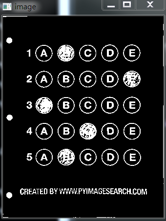
　　这效果是相当的好，我们不需要再对图像做其他任何处理，直接获取图像轮廓，如下：

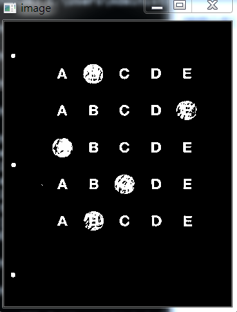
　　这清晰的，ABCDE都能看见。实在是夸张。。。。。

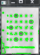
　　后面我们就不展示第一个图了，直接展示涂答题卡的。拿到轮廓之后，我们需要筛选出涂了答题卡的，首先我们拿到每个轮廓，我们比对一下涂了和没涂的效果，如下图所示：

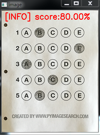
　　最后我们对比正确答案，和上面一样，我们将正确答案标记出来，使用绿色，错误答案也标记出来，使用红色。然后展示一下。

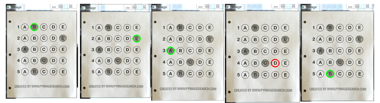
　　我们发现有四个绿的（正确的），一个红的（错误的），所以得到最终准确率为80%，我们展示在答题卡上如下：

　　再看一个：

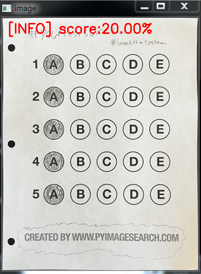
　　OK，标准的答题卡项目也完成了。

2.4.3 部分代码展示

　　需要全部代码，请去我的GitHub拿，这里展示一点重要的代码，如下：

#_*_coding:utf-8_*_
import numpy as np
import cv2
 
 
def sorted_contours(cnts, method='left-to-right'):
    if method == 'top-to-bottom':
        cnts = sorted(cnts, key=lambda x:cv2.boundingRect(x)[1])
 
    elif method == 'left-to-right':
        cnts = sorted(cnts, key=lambda x:cv2.boundingRect(x)[0])
 
    return cnts
 
 
 
# 正确答案
ANSWER_KEY = {0:1, 1:4, 2:0, 3:3, 4:1}
 
def answersheet_comparison(filename):
    '''
        对变换后的图像进行操作（wraped），构造mask
        根据有无填涂的特性，进行位置的计算
    '''
    img = cv2.imread(filename)
    # print(img.shape)   
    gray = cv2.cvtColor(img, cv2.COLOR_BGR2GRAY)
    thresh = cv2.threshold(gray, 0, 255,cv2.THRESH_BINARY_INV | cv2.THRESH_OTSU)[1] 
    # show(thresh)
    thresh_Contours = thresh.copy()
    # 找到每一个圆圈轮廓
    cnts = cv2.findContours(thresh.copy(), cv2.RETR_EXTERNAL, cv2.CHAIN_APPROX_SIMPLE)[0]
    # cv2.drawContours(thresh_Contours, cnts, -1, (0, 0, 255), 3)
    # show(thresh_Contours)
    questionCnts = []
    # 遍历
    for c in cnts:
        # 计算比例和大小
        (x, y, w, h) = cv2.boundingRect(c)
        ar = w / float(h)
        # 根据实际情况指定标准
        if w>=20 and h>=20 and ar>=0.9 and ar<=1.1:
            questionCnts.append(c)
 
    # cv2.drawContours(thresh_Contours, questionCnts, -1, (0, 0, 255), 3)[0]
    # show(thresh_Contours)
 
    print('筛选出来的轮廓有： ', len(questionCnts))
    # 按照从上到下进行排序
    questionCnts = sorted_contours(questionCnts, method='top-to-bottom')
    correct = 0
    # 每排有5个选项
    print('筛选出来的轮廓有： ', len(questionCnts))
    for (q, i) in enumerate(np.arange(0, len(questionCnts), 5)):
        # 排序
        cnts = sorted_contours(questionCnts[i:i+5])
        bubbled = None
        # 遍历每一个结果
        for (j, c) in enumerate(cnts):
            # 使用mask来判断结果
            mask = np.zeros(thresh.shape, dtype='uint8')
            cv2.drawContours(mask, [c], -1, 255, -1)  # -1 表示填充
            # 通过计算非零点数量来算是否选择这个答案
            mask = cv2.bitwise_and(thresh, thresh, mask=mask)
            # show(mask)
            total = cv2.countNonZero(mask)
            # print('total is   ',total)  # 涂了颜色的 黑色总值很大  大于600 而没有涂的小于300
            # total is    716   total is    299
 
            # 通过阈值判断
            if bubbled is None or total > bubbled[0]:
                bubbled = (total, j)
 
        # 对比正确答案
        color = (0, 0, 255)
        k = ANSWER_KEY[q]
        # 判断正确
        if k == bubbled[1]:
            color = (0, 255, 0)
            correct +=1
 
        # 绘图
        res = img.copy()
        cv2.drawContours(res, [cnts[k]], -1, color, 3)
        show(res)
 
    # score = (correct / 5.0)*100
    # print("[INFO] score: {:.2f}%".format(score))
    # cv2.putText(img, "[INFO] score:{:.2f}%".format(score), (10, 30),
    # cv2.FONT_HERSHEY_SIMPLEX, 0.9, (0, 0, 255), 2)
    # show(img)
 
if __name__ == '__main__':
    filename = r'test_01.png'
    answersheet_comparison(filename)

参考文献：https://www.pyimagesearch.com/2014/09/01/build-kick-ass-mobile-document-scanner-just-5-minutes/

https://blog.csdn.net/weixin_30666753/article/details/99054383

https://www.cnblogs.com/my-love-is-python/archive/2004/01/13/10439224.html

posted @ 2020-11-11 09:07 战争热诚阅读(16641) 评论(5) 编辑收藏举报

刷新页面返回顶部

登录后才能查看或发表评论，立即登录或者逛逛博客园首页

公告

昵称：战争热诚
园龄： 7年6个月
粉丝： 2188
关注： 30

+加关注

2025年3月

日

一

二

三

四

五

六

战争热诚

OpenCV实战（4）——文档扫描OCR识别&答题卡识别判卷（文档扫描，图像矫正，透视变换，OCR识别）

如果需要处理的原图及代码，请移步小编的GitHub地址

项目实战1——文档扫描OCR识别

1.1，文档轮廓提取

1.2，透视变换（摆正图像）

1.2.1，cv2.getPerspectiveTransform()

1.2.2，cv2.warpPerspective()

1.2.3 cv2.perspectiveTransform()

1.2.4 摆正图像

1.2.5 其他图片矫正实践

1.3，OCR识别

深入学习使用ocr算法识别图片中文字的方法

深入学习Tesseract-ocr识别中文并训练字库的方法

1.3.1 通过Python使用tesseract的坑

1.3.2 OCR识别

1.4，完整代码

项目实战2——答题卡识别判卷

2.1 扫描答题卡及透视变换

2.2 根据正确答案和图卡判断正确率

2.3 部分代码展示

2.4 高清答题卡识别

2.4.1 cv2.countNonZero()函数

2.4.2 根据正确答案和图卡判断正确率（图片清晰版）

2.4.3 部分代码展示

公告

我的标签

随笔档案

阅读排行榜

评论排行榜

推荐排行榜

最新评论

喜欢请打赏