用python进行数据分析--引言

前言

这是用学习《用python进行数据分析》的连载。这篇博客记录的是学习第二章引言部分的内容

 

内容

一、分析usa.org的数据

（1）载入数据

import json

if __name__ == "__main__":
    # load data
    path = "../../datasets/bitly_usagov/example.txt"
    with open(path) as data:
        records = [json.loads(line) for line in data]

（2）计算数据中不同时区的数量

1、复杂的方式

# define the count function
def get_counts(sequence):
    counts = {}
    for x in sequence:
        if x in counts:
            counts[x] += 1
        else:
            counts[x] = 1
    return counts

2.简单的方式

from collections import defaultdict

# to simple the count function
def simple_get_counts(sequence):
    # initialize the all value to zero
    counts = defaultdict(int)
    for x in sequence:
        counts[x] += 1
    return counts

简单之所以简单是因为它引用了defaultdicta函数，初始化了字典中的元素，将其值全部初始化为0，就省去了判断其值是否在字典中出现的过程

（3）获取出现次数最高的10个时区名和它们出现的次数

1.复杂方式

# get the top 10 timezone which value is biggest
def top_counts(count_dict, n=10):
    value_key_pairs = [(count, tz) for tz, count in count_dict.items()]
    # this sort method is asc
    value_key_pairs.sort()
    return value_key_pairs[-n:]

# get top counts by get_count function
counts = simple_get_counts(time_zones)
top_counts = top_counts(counts)

2.简单方式

from collections import Counter

# simple the top_counts method
def simple_top_counts(timezone, n=10):
    counter_counts = Counter(timezone)
    return counter_counts.most_common(n)
simple_top_counts(time_zones)

简单方式之所以简单，是因为他利用了collections中自带的counter函数，它能够自动的计算不同值出现的次数，并且不需要先计算counts

（4）利用pylab和dataframe画出不同timezone的出现次数，以柱状图的形式。

from pandas import DataFrame, Series
import pandas as pd
import numpy as np
import pylab as pyl

# use the dataframe to show the counts of timezone
def show_timezone_data(records):
    frame = DataFrame(records)
    clean_tz = frame['tz'].fillna("Missing")
    clean_tz[clean_tz == ''] = 'Unknown'
    tz_counts = clean_tz.value_counts()
    tz_counts[:10].plot("barh", rot=0)
    pyl.show()

以下是结果图：

 

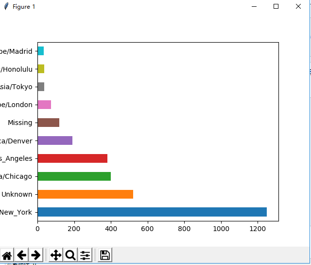
我刚开始的时候，能够执行代码，但是一直显示不出这个图。后来我查阅了资料发现是因为，我用的是pycharm，它是一个编辑器，不处于pylab模式，所以你需要先引入pylab模块，然后执行 pylab.show()指令才能够使这个图出现。

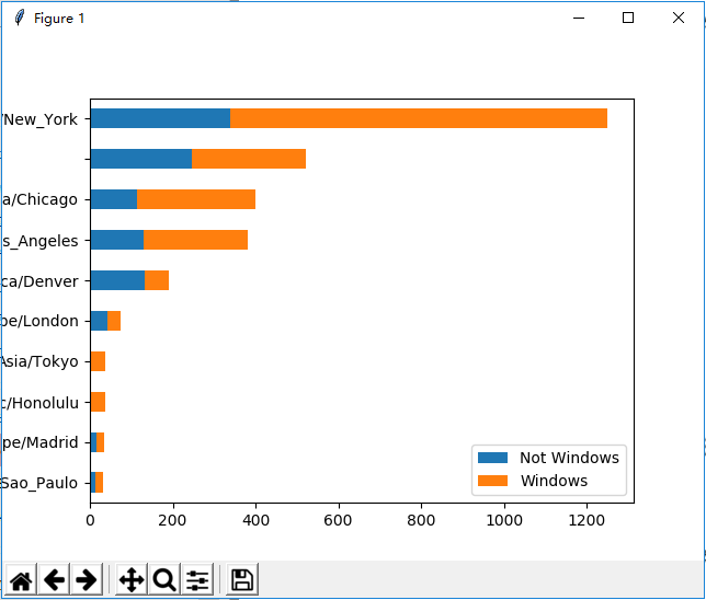
（5）利用pylab和dataframe画出不同的timezone的window的分布情况

 

# use the dataframe to show the character of timezone and windows
def show_timezone_winows(records):
    frame = DataFrame(records)
    # results = Series([x.split()[0] for x in frame.a.dropna()])
    cframe = frame[frame.a.notnull()]
    operatine_system = np.where(cframe['a'].str.contains("Windows"), "Windows", "Not Windows")
    by_tz_os = cframe.groupby(["tz", operatine_system])
    agg_counts = by_tz_os.size().unstack().fillna(0)
    indexer = agg_counts.sum(1).argsort()
    count_subset = agg_counts.take(indexer)[-10:]
    count_subset.plot(kind='barh', stacked=True)
    pyl.show()
    # let the sum to be 1
    normed_subset = count_subset.div(count_subset.sum(1), axis=0)
    normed_subset.plot(kind='barh', stacked=True)
    pyl.show()

 

 

 

没有归一化前的结果图：

 

归一化后的结果图：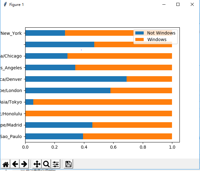

 

二、分析movielens的数据

（1）读取数据

users：记录了用户信息， ratings:记录了用户的评分信息， movies:记录了电影信息

import pandas as pd

# read the three tables
unames = ['user_id', 'gender', 'age', 'occupation', 'zip']
users = pd.read_table("../../datasets/movielens/users.dat", sep='::', header=None, names=unames)

rnames = ['user_id', 'movie_id', 'rating', 'timestamp']
ratings = pd.read_table("../../datasets/movielens/ratings.dat", sep='::', header=None, names=rnames)

mnames = ['movie_id', 'title', 'genres']
movies = pd.read_table('../../datasets/movielens/movies.dat', sep="::", header=None, names=mnames)

 

（2）合并数据

数据的合并用到了pandas中merge函数，它能够直接根据数据对象中列名直接推断出哪些列是外键

  # merge data
    return pd.merge(pd.merge(users, ratings), movies)

(3) 查询同一电影不同性别的评分

def mean_score(data):
    '''
    print the mean rating of the same title between genders
    :param data:the data source
    :return:
    '''
    mean_ratings = data.pivot_table(values='rating', index=['title'], columns='gender', aggfunc='mean')
    rating_by_title = data.groupby('title').size()
    active_titles = rating_by_title.index[rating_by_title >= 250]
    mean_ratings = mean_ratings.ix[active_titles]
    print(mean_ratings)

这里要特别注意的是，现在的dataframe中的pivot_table中已经没有了rows和cols这两项，并且在定义聚集值是需要指定。

#以前的代码
   mean_ratings =  data.pivot_table('rating', rows='title', cols='gender', aggfunc='mean')
#现在的代码
    mean_ratings = data.pivot_table(values='rating', index=['title'], columns='gender', aggfunc='mean')
   

（4）计算评分分歧

def diff_score(mean_ratings, data):
    '''
    calculate the diff between different group like male and female
    :param data:
    :return:
    '''
    mean_ratings['diff'] = mean_ratings['M'] - mean_ratings['F']
    # sorted the table by diff ,asc
    sorted_by_diff = mean_ratings.sort_index(by='diff')
    print("sorted by diff between male and female")
    print(sorted_by_diff[:10])
    # calculate the most diff movies by ignoring gender
    rating_std_by_title = data.groupby('title')['rating'].std()
    rating_std_by_title.sort_values(ascending=False)
    print("sorted by diff in rating")
    print(rating_std_by_title[:10])

这里要注意的是，现在的series中已经没有order这个函数了，取而代之的是sort_values和sort_index，不过作用是一样的。从以下的代码可以看到区别。

#以前的代码
rating_std_by_title.order(ascending=False)
#现在的代码
rating_std_by_title.sort_values(ascending=False)

 

三、分析婴儿姓名

（1）读取数据

def contact_data():
    '''
    contact all name in different year into one table
    :return:
    '''
    years = range(1880, 2011)
    pieces = []
    columns = ['name', 'sex', 'births']
    for year in years:
        path = "../../datasets/babynames/yob%d.txt" % year
        frame = pd.read_csv(path, names=columns)
        frame['year'] = year
        pieces.append(frame)
    data = pd.concat(pieces,ignore_index=True)
    return data

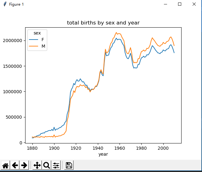
（2）画出每年不同姓名的婴儿的出生数量

def gather_function(data):
    total_births = data.pivot_table(values='births', index=['year'], columns='sex', aggfunc=sum)
    total_births.tail()
    total_births.plot(title='total births by sex and year')
    pyl.show()

结果图：

（3）获取命名次数前1000的名字

def get_top1000(group):
    return group.sort_index(by='births', ascending=False)[:1000]

def prop_function(data):
    names = data.groupby(["year", "sex"]).apply(add_prop)
    # print(np.allclose(names.groupby(['year', 'sex']).prop.sum(), 1))
    grouped = names.groupby(['year', 'sex'])
    top1000 = grouped.apply(get_top1000)
    return top1000

这里比较特别的是用了apply进行groupby函数的group方法的重写。

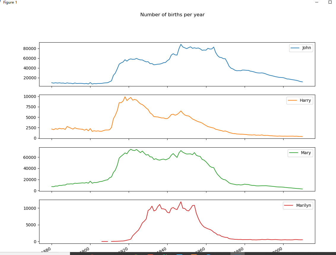
（4）分析命名趋势

def name_trend(data, top1000):
    boys = top1000[top1000.sex == 'M']
    girls = top1000[top1000.sex == 'F']
    total_births = top1000.pivot_table(values='births', index=['year'], columns='name', aggfunc=sum)
    subset = total_births[['John', 'Harry', 'Mary', 'Marilyn']]
    subset.plot(subplots=True, figsize=(12, 10), grid=False, title="Number of births per year")
    pyl.show()

分析了john,harry,mary和marilyn这四个名字在不同年份的命名趋势。

 

 （4）名字多样性的增长

有两种方式可以进行辅证

1.计算排名前1000的名字在所有名字中的占比。

def variety_growth(top1000):
    table = top1000.pivot_table(values='prop', index=['year'], columns='sex', aggfunc=sum)
    table.plot(title="sum of top1000.prop by year and sex", yticks=np.linspace(0, 1.2, 13), xticks=range(1880, 2020, 10))
    pyl.show()
    

可以得到下图：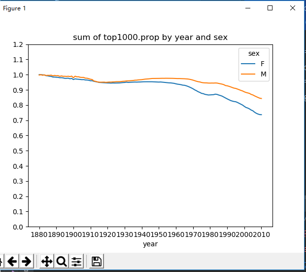

2.计算不同性别，不同年份，在top1000中需要多少个名字才能达到占比0.5

 def get_quantile_count(group, q=0.5):
    group = group.sort_index(by='prop', ascending=False)
    return group.prop.cumsum().searchsorted(q)+1

def variety_growth(top1000):
    '''
    show the plot of sum of top1000.prop by year and sex
    and the plot of number of the popular names in top 50%
    :param top1000:
    :return:
    '''
    table = top1000.pivot_table(values='prop', index=['year'], columns='sex', aggfunc=sum)
    table.plot(title="sum of top1000.prop by year and sex", yticks=np.linspace(0, 1.2, 13), xticks=range(1880, 2020, 10))
    pyl.show()
    diversity = top1000.groupby(['year', 'sex']).apply(get_quantile_count)
    diversity = diversity.unstack('sex')
    print(diversity.head())

结果如下：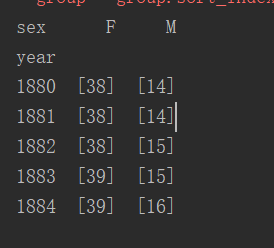

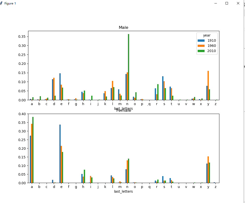
（4）最后一个字母的变革

查看不同年份，不同性别最后一个字母的占比。

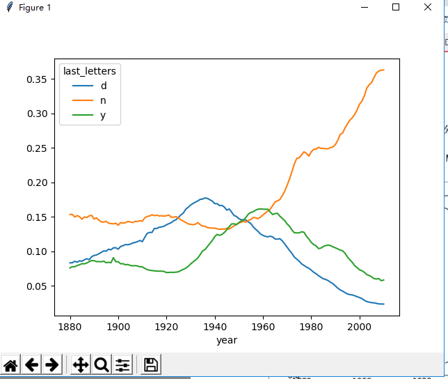
def last_name(data):
    '''
    the ratio of the character in last name by year and sex
    :param data: 
    :return: 
    '''
    get_last_letter = lambda x: x[-1]
    last_letters = data.name.map(get_last_letter)
    data['last_letters'] = last_letters
    table = data.pivot_table(values='births', index=['last_letters'], columns=['sex', 'year'], aggfunc=sum)
    subtable = table.reindex(columns=[1910, 1960, 2010], level='year')
    letter_prop = subtable/subtable.sum().astype(float)
    fig, axes = plt.subplots(2, 1, figsize=(10, 8))
    letter_prop['M'].plot(kind='bar', rot=0, ax=axes[0], title='Male')
    letter_prop['F'].plot(kind='bar', rot=0, ax=axes[1], title='Female', legend=False)
    pyl.show()
    letter_prop = table/table.sum().astype(float)
    dny_ts = letter_prop.ix[['d', 'n', 'y'], 'M'].T
    dny_ts.plot()
    pyl.show()

它的结果图如下：

 

在写这个代码的时候要注意，要加上一行 data['last_letters'] = last_letters，用来将last_letters这个列并入到data中，否则按照书上的代码执行会报错。

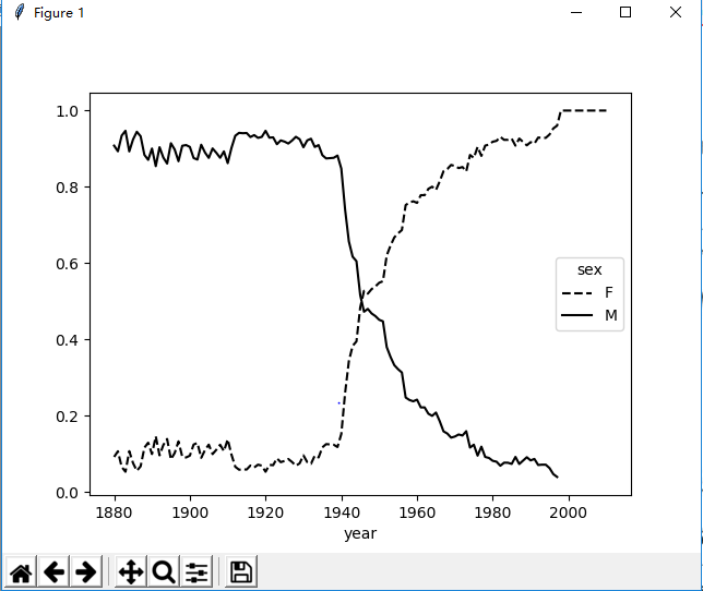
（5）变成女孩名字的男孩名字（以及相反情况）

 

def name_change_sex(top1000):
    allnames = top1000.name.unique()
    mask = np.array(['lesl' in i.lower() for i in allnames])
    lesley_like = allnames[mask]
    # filter by lesley_like
    filtered = top1000[top1000.name.isin(lesley_like)]
    table = filtered.pivot_table(values='births', index=['year'], columns='sex', aggfunc=sum)
    table = table.div(table.sum(1), axis=0)
    table.plot(style={'M': 'k-', 'F': 'k--'})
    pyl.show()

结果图：