python_数据分析与挖掘实战_客户流失预测

import matplotlib.pyplot as plt
import pandas as pd
import numpy as np
data = pd.read_csv('../../data/0307/air_data.csv')
resultfile = 'C:\\Users\\15856\\Desktop\\explore.csv'
explore = data.describe(percentiles=[], include='all').T
explore['null'] = len(data) - explore['count']
explore = explore[['null','max','min']]
explore.columns = [u'空值数',u'最大值',u'最小值']
explore.to_csv(resultfile)
from datetime import datetime
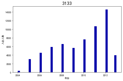
ffp = data['FFP_DATE'].apply(lambda x : datetime.strptime(x,'%Y/%m/%d'))
ffp_year = ffp.map(lambda x : x.year)
fig = plt.figure(figsize=(8,5))
plt.rcParams['font.sans-serif'] = ['SimHei']
plt.rcParams['axes.unicode_minus'] = False
plt.hist(ffp_year, bins='auto', color='#0504aa')
plt.xlabel('年份')
plt.ylabel('入会人数')
plt.title('3133',fontsize=20)
plt.show()
plt.close

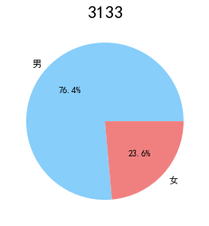
male = pd.value_counts(data['GENDER'])['男']
female = pd.value_counts(data['GENDER'])['女']
fig = plt.figure(figsize=(7,4))
plt.pie([male, female], labels=['男','女'],colors=['lightskyblue','lightcoral'],autopct='%1.1f%%')
plt.title('3133',fontsize=20)
plt.show()
plt.close

 

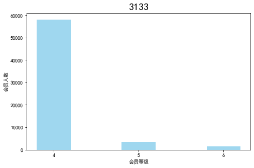
lv_four = pd.value_counts(data['FFP_TIER'])[4]
lv_five = pd.value_counts(data['FFP_TIER'])[5]
lv_six = pd.value_counts(data['FFP_TIER'])[6]
fig = plt.figure(figsize=(8,5))
plt.bar(x=range(3), height=[lv_four,lv_five,lv_six], width=0.4, alpha=0.8, color='skyblue')
plt.xticks([index for index in range(3)], ['4','5','6'])
plt.xlabel('会员等级')
plt.ylabel('会员人数')
plt.title('3133',fontsize=20)
plt.show()
plt.close

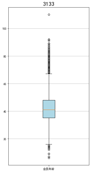
age = data['AGE'].dropna()
age = age.astype('int64')
fig = plt.figure(figsize=(5,10))    
plt.boxplot(age,
            patch_artist=True,
            labels=['会员年龄'],
            boxprops={'facecolor':'lightblue'})
plt.title('3133',fontsize=20)
plt.grid(axis='y')
plt.show()
plt.close

lte = data['LAST_TO_END']
fc = data['FLIGHT_COUNT']
sks = data['SEG_KM_SUM']
fig = plt.figure(figsize=(5,8))
plt.boxplot(lte,
            patch_artist=True,
            labels=['时长'],
            boxprops={'facecolor':'lightblue'})
plt.title('3133',fontsize=20)
plt.grid(axis='y')
plt.show()
plt.close

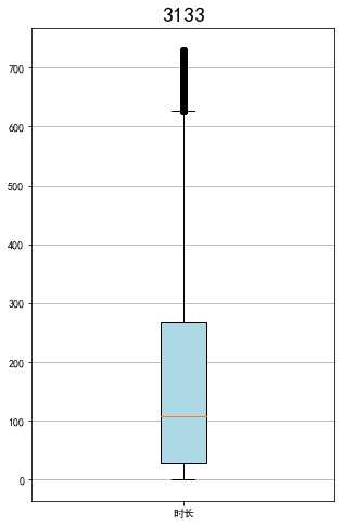
fig = plt.figure(figsize=(5,8))
plt.boxplot(fc,
            patch_artist=True,
            labels=['飞行次数'],
            boxprops={'facecolor':'lightblue'})
plt.title('3133',fontsize=20)
plt.grid(axis='y')
plt.show()
plt.close

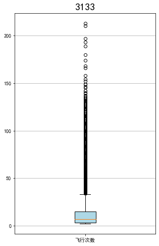
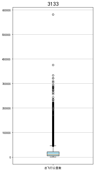
fig = plt.figure(figsize=(5,10))
plt.boxplot(sks,
            patch_artist=True,
            labels=['总飞行公里数'],
            boxprops={'facecolor':'lightblue'})
plt.title('3133',fontsize=20)
plt.grid(axis='y')
plt.show()
plt.close

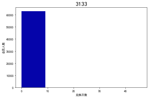
ec = data['EXCHANGE_COUNT']
fig = plt.figure(figsize=(8,5))
plt.hist(ec, bins=5, color='#0504aa')
plt.xlabel('兑换次数')
plt.ylabel('会员人数')
plt.title('3133',fontsize=20)
plt.show()
plt.close

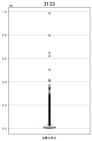
ps = data['Points_Sum']
fig = plt.figure(figsize=(5,8))
plt.boxplot(ps,
            patch_artist=True,
            labels=['总累计积分'],
            boxprops={'facecolor':'lightblue'})
plt.title('3133',fontsize=20)
plt.grid(axis='y')
plt.show()
plt.close

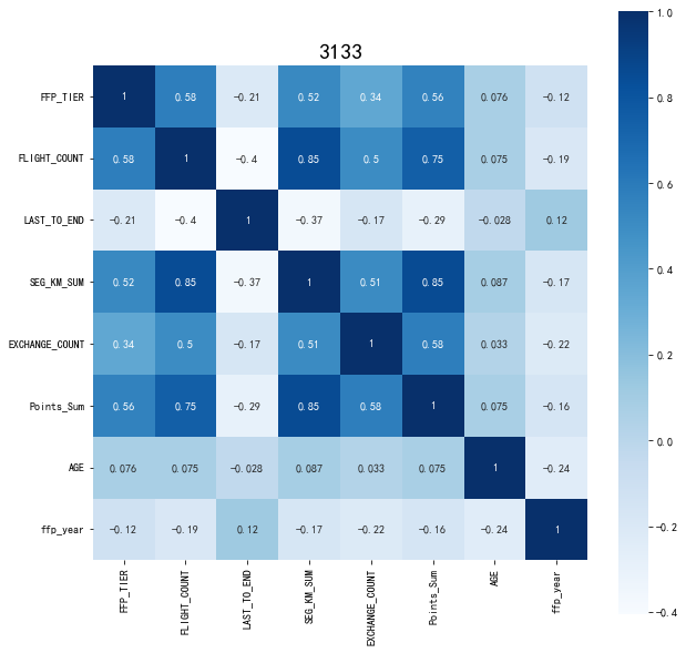
data_corr = data[['FFP_TIER','FLIGHT_COUNT','LAST_TO_END','SEG_KM_SUM','EXCHANGE_COUNT','Points_Sum']]
age1 = data['AGE'].fillna(0)
data_corr['AGE'] = age1.astype('int64')
data_corr['ffp_year'] = ffp_year
dt_corr = data_corr.corr(method='pearson')
print('相关性矩阵为：\n',dt_corr)
import seaborn as sns
plt.subplots(figsize=(10,10))
sns.heatmap(dt_corr, annot=True, vmax=1, square=True, cmap='Blues')
plt.title('3133',fontsize=20)
plt.show()
plt.close

airline_data = pd.read_csv('../../data/0307/air_data.csv')
resultfile = '../../data/0307/data_cleaned.csv'
# resultfile = 'C:\\Users\\15856\\Desktop\\data_cleaned.csv'
airline_notnull = airline_data.loc[airline_data['SUM_YR_1'].notnull() &
                                   airline_data['SUM_YR_2'].notnull(),:]
index1 = airline_notnull['SUM_YR_1'] != 0
index2 = airline_notnull['SUM_YR_2'] != 0
index3 = (airline_notnull['SEG_KM_SUM'] > 0) & (airline_notnull['avg_discount'] != 0)
index4 = airline_notnull['AGE'] > 100
airline = airline_notnull[(index1 | index2) & index3 & ~index4]
airline.to_csv(resultfile)
airline = pd.read_csv('../../data/0307/data_cleaned.csv')
airline_selection = airline[['FFP_DATE','LOAD_TIME','LAST_TO_END','FLIGHT_COUNT','SEG_KM_SUM','avg_discount']]
print('筛选的属性前5行为：\n',airline_selection.head())
L = pd.to_datetime(airline_selection['LOAD_TIME']) - pd.to_datetime(airline_selection['FFP_DATE'])
L = L.astype('str').str.split().str[0]
L = L.astype('int')/30
# L = L.astype('str')
airline_features = pd.concat([L,airline_selection.iloc[:,2:]], axis=1)
airline_features.columns = airline_features.columns.astype(str)
print('构建的LRFMC属性前5行为：\n',airline_features.head())

from sklearn.preprocessing import StandardScaler
data = StandardScaler().fit_transform(airline_features)
np.savez('../../data/0307/airline_scale.npz',data)
print('标准化后LRFMC 5个属性为：\n',data[:5,:])
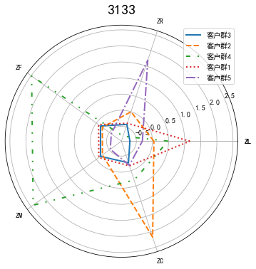
from sklearn.cluster import KMeans
airline_scale = np.load('../../data/0307/airline_scale.npz')['arr_0']
k = 5
kmeans_model = KMeans(n_clusters=k,  random_state=123)
fit_kmeans = kmeans_model.fit(airline_scale)
kmeans_cc = kmeans_model.cluster_centers_
kmeans_labels = kmeans_model.labels_
r1 = pd.Series(kmeans_model.labels_).value_counts()
cluster_center = pd.DataFrame(kmeans_model.cluster_centers_,columns=['ZL','ZR','ZF','ZM','ZC'])
cluster_center.index = pd.DataFrame(kmeans_model.labels_).drop_duplicates().iloc[:,0]
print(cluster_center)
labels = ['ZL','ZR','ZF','ZM','ZC']
# labels = labels.append('ZL')
legen = ['客户群' + str(i + 1) for i in cluster_center.index]
lstype = ['-','--',(0,(3,5,1,5,1,5)),':','-.']
kinds = list(cluster_center.iloc[:,0])


cluster_center = pd.concat([cluster_center,cluster_center[['ZL']]], axis=1)
centers = np.array(cluster_center.iloc[:,0:])

n = len(labels)
angle = np.linspace(0, 2*np.pi, n, endpoint=False)
# print([angle[0]])
angle = np.concatenate((angle, [angle[0]]))
labels = np.concatenate((labels, [labels[0]]))
fig = plt.figure(figsize=(8,6))
ax = fig.add_subplot(111,polar=True)
plt.rcParams['font.sans-serif'] = ['SimHei']
plt.rcParams['axes.unicode_minus'] = False

# print(cluster_center)
# print(centers)
# print(angle)

for i in range(len(kinds)):
    ax.plot(angle, centers[i], linestyle=lstype[i], linewidth=2, label=kinds[i])
# ax.plot(angle, centers, linestyle=lstype[i], linewidth=2, label=kinds[i])
ax.set_thetagrids(angle*180/np.pi,labels)
plt.title('3133',fontsize=20)
plt.legend(legen)
plt.show()
plt.close

import matplotlib.pyplot as plt
import pandas as pd
import numpy as np
import matplotlib.ticker as mtick
data = pd.read_csv('../../data/0307/WA_Fn-UseC_-Telco-Customer-Churn.csv')

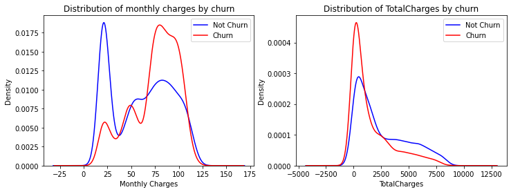
# #用密度图展现月消费、总消费与流失的关系
fig, ax = plt.subplots(1,2,figsize=(12,4))
data.MonthlyCharges[data['Churn'] == 'No'].plot(kind = 'kde',color ='blue',ax=ax[0])
data.MonthlyCharges[data['Churn'] == 'Yes'].plot(kind = 'kde',color ='red',ax=ax[0])
ax[0].legend(["Not Churn","Churn"],loc='upper right')
ax[0].set_ylabel('Density')
ax[0].set_xlabel('Monthly Charges')
ax[0].set_title('Distribution of monthly charges by churn')
ax[0].set_ylim(0)

#总消费需要转化数据类型，并把空值填充为0
data['TotalCharges'] = data['TotalCharges'].replace(" ", 0).astype('float')
data.TotalCharges[data['Churn'] == 'No'].plot(kind = 'kde',color ='blue',ax=ax[1])
data.TotalCharges[data['Churn'] == 'Yes'].plot(kind = 'kde',color ='red',ax=ax[1])
ax[1].legend(["Not Churn","Churn"],loc='upper right')
ax[1].set_ylabel('Density')
ax[1].set_xlabel('TotalCharges')
ax[1].set_title('Distribution of TotalCharges by churn')
ax[1].set_ylim(0)

# 对数据进行虚拟变量处理，也叫哑变量和离散特征编码，可用来表示分类变量、非数量因素可能产生的影响。
data_xy = data.drop(['customerID','gender','PhoneService','MultipleLines'],axis=1)
data_xy['Churn'].replace(to_replace='Yes', value=1, inplace=True)
data_xy['Churn'].replace(to_replace='No',  value=0, inplace=True)
data_dummies = pd.get_dummies(data_xy)

# 归一化数据
from sklearn.preprocessing import StandardScaler

standard = StandardScaler()
standard.fit(data_dummies[['tenure','MonthlyCharges','TotalCharges']])

data_dummies[['tenure','MonthlyCharges','TotalCharges']] = standard.transform(data_dummies[['tenure','MonthlyCharges','TotalCharges']])

#划分数据集
from sklearn.model_selection import train_test_split

X = data_dummies.drop('Churn', axis=1)
y = data_dummies['Churn']

X_train, X_test, y_train, y_test = train_test_split(X, y, test_size=0.3, random_state=101)

from sklearn.svm import SVC #支持向量机
from sklearn.linear_model import LogisticRegression #逻辑回归
from sklearn.naive_bayes import GaussianNB#朴素贝叶斯
from sklearn.tree import DecisionTreeClassifier#决策树分类器

from sklearn.metrics import recall_score,f1_score,precision_score, accuracy_score
Classifiers = [['SVM',SVC()],
              ['LogisticRegression',LogisticRegression()],
              ['GaussianNB',GaussianNB()],
              ['DecisionTreeClassifier',DecisionTreeClassifier()]]

Classify_results = []
names = []
prediction = []
for name ,classifier in Classifiers:
    classifier.fit(X_train,y_train)#训练这4个模型
    y_pred = classifier.predict(X_test)#预测这4个模型
    
    recall = recall_score(y_test,y_pred)#评估这四个模型的召回率
    precision = precision_score(y_test,y_pred)#评估这四个模型的精确率
    f1 = f1_score(y_test,y_pred)#评估这四个模型的f1分数
    acc = accuracy_score(y_test, y_pred)
    class_eva = pd.DataFrame([recall,precision,f1,acc])#将召回率、精确率和f1分数放在df中，方便接下来对比
    Classify_results.append(class_eva)
    name = pd.Series(name)
    names.append(name)
    y_pred = pd.DataFrame(y_pred)
    prediction.append(y_pred)
    
    
    pred = y_pred.values
    test = y_test.values
    i = 0
    sum = 0
    lost = 0
    norm = 0
    wlost = 0
    wnorm = 0
    for j in test:
        if(j == pred[i]):
            sum += 1
#             正确预测保留
            if( j == 0 ):
                norm += 1
#             正确预测流失
            elif( j == 1):
                lost += 1
        else:
#             错误预测保留
            if( j == 0 ):
                wnorm += 1
#             错误预测流失
            elif( j == 1):
                wlost += 1
        i = i + 1
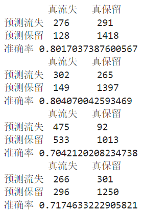
    print('\t真流失\t真保留')
    print('预测流失\t',lost,'\t',wlost)
    print('预测保留\t',wnorm,'\t',norm)
    print('准确率',sum/len(pred)) 

names = pd.DataFrame(names)
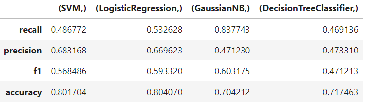
result = pd.concat(Classify_results,axis=1)
result.columns = names
result.index=[['recall','precision','f1','accuracy']]
result