猫狗识别
import os

import tensorflow.compat.v1 as tf
tf.disable_v2_behavior()
from PIL import Image
import matplotlib.pyplot as plt
import numpy as np
import cv2
def get_files(file_dir):
    cats=[] #猫的图片 列表
    lable_cats=[] #猫的标签 列表
    dogs=[] #狗的图片 列表
    lable_dogs=[]  #狗的标签 列表

    #os.listdir为列出路径内的所有文件
    for file in os.listdir(file_dir):
        name = file.split('.')   #将每一个文件名都进行分割,以.分割
        #这样文件名 就变成了三部分 name的形式 [‘dog’,‘9981’,‘jpg’]
        if name[0]=='cat':
            cats.append(file_dir+file)
            #在定义的cats列表内添加图片路径,由文件夹的路径+文件名组成
            lable_cats.append(0) #在猫的标签列表中添加对应图片的标签,猫的标签为0,狗为1
        else:
            dogs.append(file_dir+file)
            lable_dogs.append(1)
    print('There are %d cats\nThere are %d dogs' %(len(cats), len(dogs)))   #打印猫和狗的数量

    image_list = np.hstack((cats, dogs))  #将猫和狗的列表合并为一个列表
    label_list = np.hstack((lable_cats, lable_dogs)) #将猫和狗的标签列表合并为一个列表

    #将两个列表构成一个数组
    temp=np.array([image_list,label_list])
    temp=temp.transpose() #将数组矩阵转置
    np.random.shuffle(temp) #将数据打乱顺序,不再按照前边全是猫,后面全是狗这样排列
    image_list=list(temp[:,0]) #图片列表为temp 数组的第一个元素
    label_list = list(temp[:, 1]) #标签列表为temp数组的第二个元素
    label_list = [int(i) for i in label_list] #转换为int类型
    #返回读取结果,存放在image_list,和label_list中
    return image_list, label_list
def get_batch(image,label,image_W,image_H,batch_size,capacity):
    #数据转换
    image = tf.cast(image, tf.string)   #将image数据转换为string类型
    label = tf.cast(label, tf.int32)    #将label数据转换为int类型
    #入队列
    input_queue = tf.train.slice_input_producer([image, label])
    #取队列标签 张量
    label = input_queue[1]
    #取队列图片 张量
    image_contents = tf.read_file(input_queue[0])
    #解码图像,解码为一个张量
    image = tf.image.decode_jpeg(image_contents, channels=3)
    #对图像的大小进行调整,调整大小为image_W,image_H
    image = tf.image.resize_image_with_crop_or_pad(image, image_W, image_H)
    #对图像进行标准化
    image = tf.image.per_image_standardization(image)

    #等待出队
    image_batch, label_batch = tf.train.batch([image, label],
                                              batch_size= batch_size,
                                              num_threads= 64,
                                              capacity = capacity)
    label_batch = tf.reshape(label_batch, [batch_size]) #将label_batch转换格式为[]
    image_batch = tf.cast(image_batch, tf.float32)   #将图像格式转换为float32类型
    return image_batch, label_batch  #返回所处理得到的图像batch和标签batch
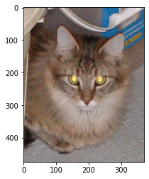
import matplotlib.pyplot as plt

BATCH_SIZE = 2
CAPACITY = 256
IMG_W = 208
IMG_H = 208

train_dir = './dataset/dc/train/'
image_list, label_list = get_files(train_dir)   #读取数据和标签
image_batch, label_batch = get_batch(image_list, label_list, IMG_W, IMG_H, BATCH_SIZE, CAPACITY)    #将图片分批次

#开启会话,使用try--except--finally结构来执行队列操作
with tf.Session() as sess:
    i = 0
    coord = tf.train.Coordinator()
    threads = tf.train.start_queue_runners(coord=coord)

    try:
        while not coord.should_stop() and i<2:

            img, label = sess.run([image_batch, label_batch])

            # just test one batch
            for j in np.arange(BATCH_SIZE):
                print('label: %d' %label[j])  #j-index of quene of Batch_size
                plt.imshow(img[j,:,:,:])
                plt.show()
            i+=1

    except tf.errors.OutOfRangeError:
        print('done!')
    finally:
        coord.request_stop()
    coord.join(threads)
def inference(images, batch_size, n_classess):
    """
    第一个卷积层
    """
    # tf.variable_scope() 主要结合 tf.get_variable() 来使用,实现变量共享。下次调用不用重新产生,这样可以保存参数
    with tf.variable_scope('conv1') as scope:         #初始化权重,[3,3,3,16]
        weights = tf.get_variable('weights', shape = [3, 3, 3, 16], dtype = tf.float32,
                                  initializer = tf.truncated_normal_initializer(stddev=0.1, dtype=tf.float32))
        #初始化偏置,16个
        biases = tf.get_variable('biases', shape=[16], dtype = tf.float32,
                                 initializer = tf.constant_initializer(0.1))
        conv = tf.nn.conv2d(images, weights, strides=[1,1,1,1], padding='SAME')
        # 将偏置加在所得的值上面
        pre_activation = tf.nn.bias_add(conv, biases)
        # 将计算结果通过relu激活函数完成去线性化
        conv1 = tf.nn.relu(pre_activation, name= scope.name)

    """
    池化层
    """
    with tf.variable_scope('pooling1_lrn') as scope:
        # tf.nn.max_pool实现了最大池化层的前向传播过程,参数和conv2d类似,ksize过滤器的尺寸
        pool1 = tf.nn.max_pool(conv1, ksize=[1,3,3,1],strides=[1,2,2,1],padding='SAME',name='poolong1')
        # 局部响应归一化(Local Response Normalization),一般用于激活,池化后的一种提高准确度的方法。
        norm1 = tf.nn.lrn(pool1, depth_radius=4, bias=1, alpha=0.001/9.0, beta=0.75, name='norm1')


    """
    第二个卷积层
    """
    # 计算过程和第一层一样,唯一区别为命名空间
    with tf.variable_scope('conv2') as scope:
        weights = tf.get_variable('weights', shape=[3,3,16,16], dtype=tf.float32, initializer=tf.truncated_normal_initializer(stddev=0.1,dtype=tf.float32))
        biases = tf.get_variable('biases',
                                 shape=[16],
                                 dtype=tf.float32,
                                 initializer=tf.constant_initializer(0.1))
        conv = tf.nn.conv2d(norm1, weights, strides=[1,1,1,1],padding='SAME')
        pre_activation = tf.nn.bias_add(conv, biases)
        conv2 = tf.nn.relu(pre_activation, name='conv2')


    """
    第二池化层
    """
    with tf.variable_scope('pooling2_lrn') as scope:
        norm2 = tf.nn.lrn(conv2, depth_radius=4,bias=1,alpha=0.001/9,beta=0.75,name='norm2')
        pool2 = tf.nn.max_pool(norm2, ksize=[1,3,3,1],strides=[1,1,1,1],padding='SAME',name='pooling2')


    """
    local3 全连接层
    """
    with tf.variable_scope('local3') as scope:
        # -1代表的含义是不用我们自己指定这一维的大小,函数会自动计算
        reshape = tf.reshape(pool2, shape=[batch_size, -1])
        # 获得reshape的列数,矩阵点乘要满足列数等于行数
        dim = reshape.get_shape()[1].value
        weights = tf.get_variable('weights', shape=[dim,128],dtype=tf.float32,initializer=tf.truncated_normal_initializer(stddev=0.005,dtype=tf.float32))
        biases = tf.get_variable('biases',shape=[128], dtype=tf.float32,initializer=tf.constant_initializer(0.1))
        local3 = tf.nn.relu(tf.matmul(reshape, weights) + biases, name=scope.name)


    """
    local4 全连接层
    """
    with tf.variable_scope('local4') as scope:
        weights = tf.get_variable('weights',shape=[128,128],dtype=tf.float32,initializer=tf.truncated_normal_initializer(stddev=0.005,dtype=tf.float32))
        biases = tf.get_variable('biases', shape=[128],dtype=tf.float32, initializer=tf.constant_initializer(0.1))
        local4 = tf.nn.relu(tf.matmul(local3,weights) + biases, name = 'local4')


    """
    lsoftmax逻辑回归
    将前面的全连接层输出,做一个线性回归,计算出每一类的得分,在这里是2类
    所以这个层输出的是2个得分
    """
    with tf.variable_scope('softmax_linear') as scope:
        weights = tf.get_variable('softmax_linear',shape=[128, n_classess],dtype=tf.float32,initializer=tf.truncated_normal_initializer(stddev=0.005,dtype=tf.float32))
        biases = tf.get_variable('biases',shape=[n_classess],dtype=tf.float32,initializer=tf.constant_initializer(0.1))
        softmax_linear = tf.add(tf.matmul(local4, weights),biases,name='softmax_linear')
    return softmax_linear
def losses(logits, labels):
    with tf.variable_scope('loss') as scope:
        # 计算使用了softmax回归后的交叉熵损失函数
        # logits表示神经网络的输出结果,labels表示标准答案
        cross_entropy = tf.nn.sparse_softmax_cross_entropy_with_logits(logits=logits, labels=labels,name='xentropy_per_example')
        # 求cross_entropy所有元素的平均值
        loss = tf.reduce_mean(cross_entropy, name='loss')
        # 对loss值进行标记汇总,一般在画loss, accuary时会用到这个函数。
        tf.summary.scalar(scope.name+'/loss',loss)
    return loss
def trainning(loss, learning_rate):
    with tf.name_scope('optimizer'):
        # 在训练过程中,先实例化一个优化函数,比如tf.train.GradientDescentOptimizer,并基于一定的学习率进行梯度优化训练
        optimizer = tf.train.AdamOptimizer(learning_rate=learning_rate)
        # 设置一个用于记录全局训练步骤的单值
        global_step = tf.Variable(0, name='global_step',trainable=False)
        # 添加操作节点,用于最小化loss,并更新var_list,返回为一个优化更新后的var_list,如果global_step非None,该操作还会为global_step做自增操作
        train_op = optimizer.minimize(loss, global_step=global_step)
    return train_op
def evaluation(logits, labels):
    with tf.variable_scope('accuracy') as scope:
        correct = tf.nn.in_top_k(logits,labels,1)
        # 计算预测的结果和实际结果的是否相等,返回一个bool类型的张量
        # K表示每个样本的预测结果的前K个最大的数里面是否含有target中的值。一般都是取1。
        # 转换类型
        correct = tf.cast(correct, tf.float16)
        accuracy = tf.reduce_mean(correct)
        #取平均值,也就是准确率
        # 对准确度进行标记汇总
        tf.summary.scalar(scope.name+'/accuracy',accuracy)
    return accuracy
import os
import numpy as np
import tensorflow.compat.v1 as tf
tf.disable_v2_behavior()
from PIL import Image
import matplotlib.pyplot as plt
N_CLASSES = 2 # 二分类问题,只有是还是否,即0,1
IMG_W = 208 #图片的宽度
IMG_H = 208 #图片的高度
BATCH_SIZE = 16 #批次大小
CAPACITY = 2000  # 队列最大容量2000
MAX_STEP = 5000 #最大训练步骤
learning_rate = 0.0001  #学习率
def run_training():
    """
    ##1.数据的处理
    """
    # 训练图片路径
    train_dir = './dataset/dc/train/'
    # 输出log的位置
    logs_train_dir = './model/'
    # 模型输出
    train_model_dir = './model/'
    # 获取数据中的训练图片 和 训练标签
    train, train_label = get_files(train_dir)
    # 获取转换的TensorFlow 张量
    train_batch, train_label_batch = get_batch(train,train_label,IMG_W,IMG_H,BATCH_SIZE,CAPACITY)


    """
    ##2.网络的推理
    """
    # 进行前向训练,获得回归值
    train_logits = inference(train_batch, BATCH_SIZE, N_CLASSES)

    """
    ##3.定义交叉熵和 要使用的梯度下降的 优化器
    """
    # 计算获得损失值loss
    train_loss = losses(train_logits, train_label_batch)
    # 对损失值进行优化
    train_op = trainning(train_loss, learning_rate)

    """
    ##4.定义后面要使用的变量
    """
    # 根据计算得到的损失值,计算出分类准确率
    train__acc = evaluation(train_logits, train_label_batch)
    # 将图形、训练过程合并在一起
    summary_op = tf.summary.merge_all()


    # 新建会话
    sess = tf.Session()


    # 将训练日志写入到logs_train_dir的文件夹内
    train_writer = tf.summary.FileWriter(logs_train_dir, sess.graph)
    saver = tf.train.Saver()  # 保存变量

    # 执行训练过程,初始化变量
    sess.run(tf.global_variables_initializer())


    # 创建一个线程协调器,用来管理之后在Session中启动的所有线程
    coord = tf.train.Coordinator()
    # 启动入队的线程,一般情况下,系统有多少个核,就会启动多少个入队线程(入队具体使用多少个线程在tf.train.batch中定义);
    threads = tf.train.start_queue_runners(sess=sess, coord=coord)

    """
    进行训练:
    使用 coord.should_stop()来查询是否应该终止所有线程,当文件队列(queue)中的所有文件都已经读取出列的时候,
    会抛出一个 OutofRangeError 的异常,这时候就应该停止Sesson中的所有线程了;
    """

    try:
        for step in np.arange(MAX_STEP): #从0 到 2000 次 循环
            if coord.should_stop():
                break
            _, tra_loss, tra_acc = sess.run([train_op, train_loss, train__acc])

            # 每50步打印一次损失值和准确率
            if step % 50 == 0:
                print('Step %d, train loss = %.2f, train accuracy = %.2f%%' % (step, tra_loss, tra_acc * 100.0))

                summary_str = sess.run(summary_op)
                train_writer.add_summary(summary_str, step)


            # 每2000步保存一次训练得到的模型
            if step % 2000 == 0 or (step + 1) == MAX_STEP:
                checkpoint_path = os.path.join(train_model_dir, 'model.ckpt')
                saver.save(sess, checkpoint_path, global_step=step)

    # 如果读取到文件队列末尾会抛出此异常
    except tf.errors.OutOfRangeError:
        print('Done training -- epoch limit reached')
    finally:
        coord.request_stop()
        # 使用coord.request_stop()来发出终止所有线程的命令

    coord.join(threads)            # coord.join(threads)把线程加入主线程,等待threads结束
    sess.close()                   # 关闭会话
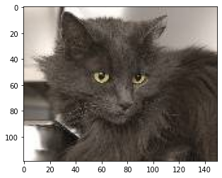
import tensorflow.compat.v1 as tf
tf.disable_v2_behavior()
import numpy as np
import math
from PIL import Image
import matplotlib.pyplot as plt
import tempfile

# 获取一张图片
def get_one_image(data):
    n = len(data)
    #训练集长度
    ind = np.random.randint(0, n)   #生成随机数
    img_dir = data[ind]    #从训练集中提取选中的图片

    image = Image.open(img_dir)
    plt.imshow(image)   #显示图片
    plt.show()
    image = image.resize([208, 208])
    image = np.array(image)
    return image

def get_one_image_file(img_dir):
    image = Image.open(img_dir)
    plt.imshow(image)   #显示图片
    plt.show()
    image = image.resize([208, 208])
    image = np.array(image)
    return image
def evaluate_one_image():
    # 数据集路径

    image_array=get_one_image_file("./dataset/dc/test/38.jpg")

    with tf.Graph().as_default():
        BATCH_SIZE = 1   # 获取一张图片
        N_CLASSES = 2  #二分类
        image = tf.cast(image_array, tf.float32)
        image = tf.image.per_image_standardization(image)
        image = tf.reshape(image, [1, 208, 208, 3])     #inference输入数据需要是4维数据,需要对image进行resize
        logit = inference(image, BATCH_SIZE, N_CLASSES)
        logit = tf.nn.softmax(logit)    #inference的softmax层没有激活函数,这里增加激活函数

        #因为只有一副图,数据量小,所以用placeholder
        x = tf.placeholder(tf.float32, shape=[208, 208, 3])
        #
        # 训练模型路径
        logs_train_dir = './model/'
        saver = tf.train.Saver()
        with tf.Session() as sess:
            # 从指定路径下载模型
            print("Reading checkpoints...")
            ckpt = tf.train.get_checkpoint_state(logs_train_dir)
            if ckpt and ckpt.model_checkpoint_path:
                global_step = ckpt.model_checkpoint_path.split('/')[-1].split('-')[-1]
                saver.restore(sess, ckpt.model_checkpoint_path)
                print('Loading success, global_step is %s' % global_step)
            else:
                print('No checkpoint file found')
            prediction = sess.run(logit, feed_dict={x: image_array})
            # 得到概率最大的索引
            max_index = np.argmax(prediction)
            if max_index==0:
                print('This is a cat with possibility %.6f' %prediction[:, 0])
            else:
                print('This is a dog with possibility %.6f' %prediction[:, 1])
def main():
    run_training()#训练模型
    evaluate_one_image()

if __name__ == '__main__':
    main()
Reading checkpoints...
INFO:tensorflow:Restoring parameters from ./model/model.ckpt-4999
Loading success, global_step is 4999
This is a dog with possibility 0.580188


再次验证发现此次判断较为准确

 浙公网安备 33010602011771号