基于libtorch的Resnet34残差网络实现——Cifar-10分类
前文我们使用libtorch实现Alexnet网络来分类Cifar-10数据集,对测试集的分类准确率达到72.02%,这个准确率对于相对Lenet-5更深的网络来说并不理想。本文我们将尝试实现Resnet34残差网络来对Cifar-10分类,看看准确率是否有提升呢?
基于libotrch的Alexnet网络实现:
基于libtorch的Alexnet深度学习网络实现——Alexnet网络结构与原理
基于libtorch的Alexnet深度学习网络实现——Cifar-10数据集分类
基于libtorch的Alexnet深度学习网络实现——Cifar-10数据集分类(提升准确率)
01
—
为什么使用残差网络?
自从Alexnet网络出来之后,人们看到Alexnet网络在Lenet-5的基础上加深的效果还是很不错的,尝到了加深网络的甜头,于是继续加深网络,但是发现网络的加深与效果的提高并不成正比:在一定程度内加深网络确实可以提高效果,但如果网络层数超过一定范围,效果不仅得不到提高,反而变差了。这是为什么呢?
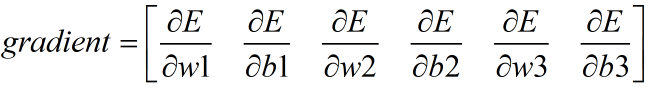
前文我们已经举例讲过误反向传播法的原理:假设有函数E=f(x),E是关于x的复合函数:

根据复合函数的求导法则,我们有:
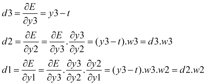
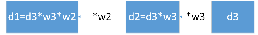
上式中d1、d2、d3就是反向传播的误差信息,它们的反向传播过程如下图:
更详细的误反向传播原理解释请参考前文:
卷积神经网络原理及其C++/Opencv实现(4)—误反向传播法
由以上原理可知,误差信息从网络末端反向传播的过程,遵循复合函数求导的链式法则,也即一个连乘的过程,而每一层网络的梯度则根据传播到该层的误差信息来计算。反向传播过程中难免有些不是很正常的误差信息(偏大或偏小),如果网络加深,连乘的次数增加,这些误差信息的异常将被放大,偏大的越来越大,造成”梯度爆炸“问题,偏小的越来接近0,造成”梯度消失“问题,这些问题都严重影响网络的训练。
残差网络,正是为解决网络加深之后导致的训练困难问题而提出来的。
02
—
残差模块原理
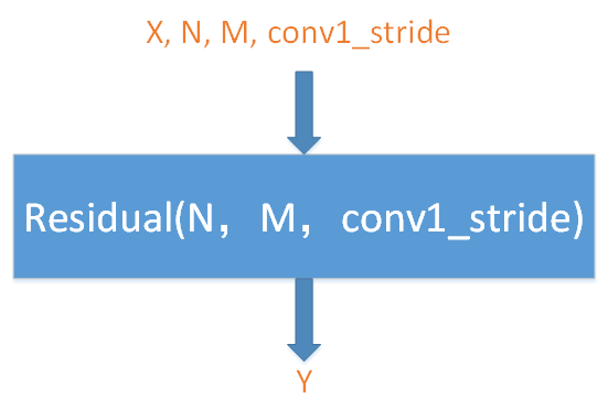
残差网络,顾名思义,其精髓在于残差模块,整个网络则由多个残差模块构成。下面我们首先讲一下残差模块的原理,其结构如下图所示,其中N为输入通道数、M为输出通道数、X为模块输入数据、Y为模块输出数据、Residual为残差信号:
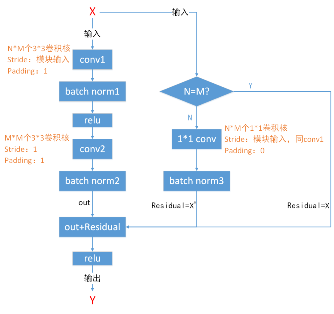
观察上图,我们发现残差模块的主要特点是把两层卷积结果与输入信号的和作为输出信号,这正是残差网络的主要特色。如下式所示,其中conv1_stride为conv1卷积层的步长,conv1_stride是模块的输入参数之一:

我们还发现:当输入通道数N与输出通道数M不相等时,残差信号Residual为输入信号X的1*1卷积结果,且1*1卷积的步长与conv1层的步长一致;当N等于M的时候,Residual则为输入信号X。
这是为什么呢?
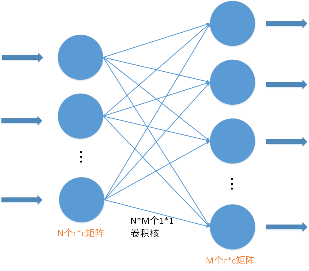
因为残差模块的输出为两层卷积结果与输入信号之和,如果输入通道数N不等于输出通道数M,那么两层卷积结果的维度(1*M*r*c)与输入信号的维度(1*N*r*c)将不一样,此时不能将两者相加,所以需要使用具有M个神经元的核为1*1的卷积层将输入信号的维度转换为(1*M*r*c),从而与两层卷积结果的维度一致。如下图所示:
在Resnet残差网络中,具有多个以上所述的残差模块,在代码实现上,我们只需要实现一次残差模块,然后多次调用该模块即可,将该模块的精简示意图如下图所示,在下文我们将使用该精简示意图来表示残差模块。
03
—
Resnet34残差网络结构
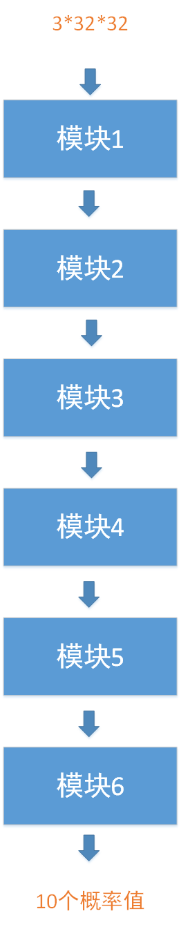
用于分类Cifar-10数据集的Resnet34残差网络可以分为6个大模块,如下图所示:
下面我们分别细说以上各个组成模块的结构。
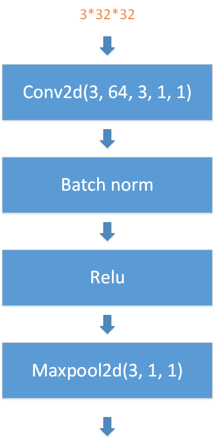
模块1:
模块1由1个卷积层、1个Batchnorm层、1个Relu层、1个pool层构成,如下图所示:
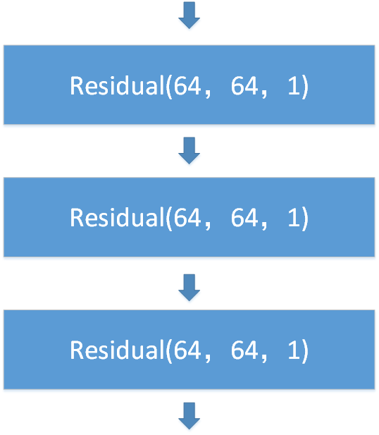
模块2:
模块2由3个残差模块构成,如下图所示:
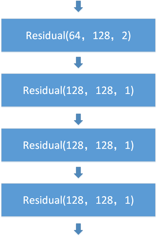
模块3:
模块3由4个残差模块构成,如下图所示:
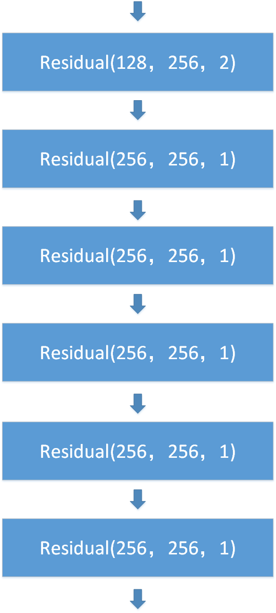
模块4:
模块4由6个残差模块构成,如下图所示:
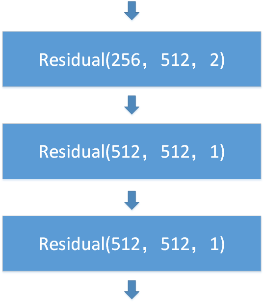
模块5:
模块5由3个残差模块构成,如下图所示:
模块6:
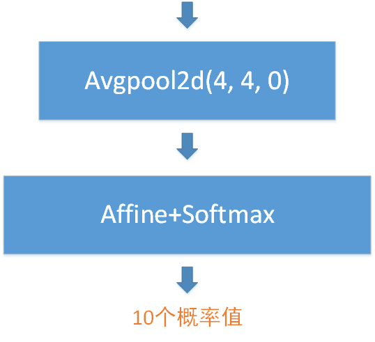
模块6由1个均值池化层和1个全连接层构成,如下图所示,其中均值池化层的池化窗口为4*4、步长为4、填充为0。
综上所述,模块1有1个卷积层、模块2~5有(3+4+6+3)*2=32个卷积层、模块6有1个全连接层,这些主要层合起来就是1+32+1=34层——Rexnet34名称的来由。
04
—
libtorch实现Resnet34残差网络
1. 残差模块的实现
由于网络中有多个残差模块,它们只是输入、输出不一样,但中间计算过程是一样的,因此可以将残差模块封装成一个Module,然后重复多次调用该Module即可:
//将残差模块封装成一个Module
struct Residual: torch::nn::Module
{
  int in_channel_r;   //输入通道数
  int out_channel_r;  //输出通道数

  //注册模块中的各个层,并设置输入通道数、输出通道数
  Residual(int in_channel, int out_channel, int _stride = 1)
  {
    conv1 = register_module("conv1", torch::nn::Conv2d(torch::nn::Conv2dOptions(in_channel, out_channel, { 3, 3 }).padding(1).stride({ _stride, _stride })));
    c1b = register_module("c1b", torch::nn::BatchNorm2d(torch::nn::BatchNorm2dOptions(out_channel).eps(1e-5).momentum(0.1).affine(true).track_running_stats(true)));
    conv2 = register_module("conv2", torch::nn::Conv2d(torch::nn::Conv2dOptions(out_channel, out_channel, { 3,3 }).padding(1).stride({ 1, 1 })));
    c2b = register_module("c2b", torch::nn::BatchNorm2d(torch::nn::BatchNorm2dOptions(out_channel).eps(1e-5).momentum(0.1).affine(true).track_running_stats(true)));
    //注意conv3 1*1卷积层与conv1卷积层的stride须保持一致
    conv3 = register_module("conv3", torch::nn::Conv2d(torch::nn::Conv2dOptions(in_channel, out_channel, { 1, 1 }).stride({ _stride, _stride })));
    c3b = register_module("c3b", torch::nn::BatchNorm2d(torch::nn::BatchNorm2dOptions(out_channel).eps(1e-5).momentum(0.1).affine(true).track_running_stats(true)));


    in_channel_r = in_channel;
    out_channel_r = out_channel;
  }


  ~Residual()
  {


  }
  //Module的前向传播函数
  torch::Tensor forward(torch::Tensor input)
  {
    namespace F = torch::nn::functional;


    auto x = conv1->forward(input);
    x = c1b->forward(x);
    x = F::relu(x);


    x = conv2->forward(x);
    x = c2b->forward(x);


    Tensor x1;
    //如果输入通道数不等于输出通道数,将对输入进行1*1卷积
    if (in_channel_r != out_channel_r)
    {
      x1 = conv3->forward(input);
      x1 = c3b->forward(x1);
    }
    else
    {
      x1 = input;
    }


    x = x + x1;  //两层卷积结果与输入信号之和
    x = F::relu(x);


    return x;
  }


  torch::nn::Conv2d conv1{ nullptr };
  torch::nn::BatchNorm2d c1b{ nullptr };   //batchnorm在卷积层之后、激活函数之前
  torch::nn::Conv2d conv2{ nullptr };
  torch::nn::BatchNorm2d c2b{ nullptr };
  torch::nn::Conv2d conv3{ nullptr };
  torch::nn::BatchNorm2d c3b{ nullptr };
};
2. Resnet34残差网络的实现
我们知道,Resnet34残差网络由模块1~模块6这六个大模块构成,那么怎么分别实现这些大模块呢?
使用libtorch中的torch::nn::Sequential,可以很方便地实现各个大模块。我们可以把torch::nn::Sequential理解成一个有顺序的容器,然后把卷积层、池化层、激活函数层、Affine层等常见Module、甚至自己手动实现的Module按照一定顺序装入该容器中,接着调用register_module函数注册该容器。这样一来我们就得到了按顺序执行的组合层,也即我们所说的大模块。
struct Resnet34 : torch::nn::Module
{
  Resnet34(int in_channel, int num_class = 10)
  {
    //注册模块1
    conv1 = register_module("conv1", torch::nn::Sequential(
      torch::nn::Conv2d(torch::nn::Conv2dOptions(in_channel, 64, { 3, 3 }).padding(1).stride({ 1, 1 })),
      torch::nn::BatchNorm2d(torch::nn::BatchNorm2dOptions(64).eps(1e-5).momentum(0.1).affine(true).track_running_stats(true)),
      torch::nn::ReLU(torch::nn::ReLUOptions(true)),
      torch::nn::MaxPool2d(torch::nn::MaxPool2dOptions({ 3, 3 }).stride({ 1, 1 }).padding(1)))
    );

    //注册模块2
    conv2 = register_module("conv2", torch::nn::Sequential(
      Residual(64, 64),    //重复调用残差模块,也相当于将多个残差模块装入顺序容器中
      Residual(64, 64),
      Residual(64, 64))
    );

    //注册模块3
    conv3 = register_module("conv3", torch::nn::Sequential(
      Residual(64, 128, 2),
      Residual(128, 128),
      Residual(128, 128),
      Residual(128, 128))
    );

    //注册模块4
    conv4 = register_module("conv4", torch::nn::Sequential(
      Residual(128, 256, 2),
      Residual(256, 256),
      Residual(256, 256),
      Residual(256, 256),
      Residual(256, 256),
      Residual(256, 256))
    );

    //注册模块5
    conv5 = register_module("conv5", torch::nn::Sequential(
      Residual(256, 512, 2),
      Residual(512, 512),
      Residual(512, 512))
    );


    //注册全连接层的Affine层,由于模块6只有1个池化层和1个全连接层,就不使用顺序容器实现了,且池化层不需要在此注册,放在前向传播函数中实现即可
    fc = register_module("fc", torch::nn::Linear(512, num_class));
  }


  ~Resnet34()
  {


  }


  //前向传播函数
  Tensor forward(Tensor input)
  {


    namespace F = torch::nn::functional;
    //模块1
    auto x = conv1->forward(input);
    //模块2
    x = conv2->forward(x);
    //模块3
    x = conv3->forward(x);
    //模块4
    x = conv4->forward(x);
    //模块5
    x = conv5->forward(x);
    //模块6
    x = F::avg_pool2d(x, F::AvgPool2dFuncOptions(4));  //池化窗口4*4,stride默认与窗口尺寸一致4*4,padding默认为0
    x = x.view({ x.size(0), -1 });  //一维展开
    x = fc->forward(x);   //Affine层,Softmax层不需要在此处计算,因为后面的CrossEntropyLoss交叉熵函数本身包含了Softmax计算


    return x;
  }


  // Use one of many "standard library" modules.
  torch::nn::Sequential conv1{ nullptr };
  torch::nn::Sequential conv2{ nullptr };
  torch::nn::Sequential conv3{ nullptr };
  torch::nn::Sequential conv4{ nullptr };
  torch::nn::Sequential conv5{ nullptr };
  torch::nn::Linear fc{ nullptr };
};
3. 数据增强实现
我们使用实现Opencv实现简单的数据增强,包括翻转、平移、缩放:
平移函数实现:
void my_pingyi(Mat src, Mat& dst, float x, float y)
{
  cv::Size dst_sz = src.size();


  cv::Mat t_mat = cv::Mat::zeros(2, 3, CV_32FC1);  //定义平移矩阵


  t_mat.at<float>(0, 0) = 1;
  t_mat.at<float>(0, 2) = x; //水平平移量
  t_mat.at<float>(1, 1) = 1;
  t_mat.at<float>(1, 2) = y; //竖直平移量


  //根据平移矩阵进行仿射变换
  cv::warpAffine(src, dst, t_mat, dst_sz, INTER_CUBIC, BORDER_REPLICATE);
}
缩放函数实现:
void my_suofang(Mat src, Mat& dst, float scale)
{
  int row = src.rows*scale;
  int col = src.cols*scale;


  if (scale < 1.0)   //缩小的情况
  {
    Mat out;
    resize(src, out, Size(col, row), INTER_CUBIC);


    int row_d = src.rows - row;
    int col_d = src.cols - col;
    int top, bottom, left, right;
    if (row_d % 2)
    {
      top = row_d / 2;
      bottom = top + 1;
    }
    else
    {
      top = row_d / 2;
      bottom = top;
    }


    if (col_d % 2)
    {
      left = col_d / 2;
      right = left + 1;
    }
    else
    {
      left = col_d / 2;
      right = left;
    }
    //填充边缘,使缩小后的图像与原图像尺寸一致
    copyMakeBorder(out, dst, top, bottom, left, right, BORDER_REPLICATE);
  }
  else if (scale > 1.0)  //放大的情况
  {
    Mat out;
    resize(src, out, Size(col, row), INTER_CUBIC);


    int x = (rand() % (col - src.cols + 1));    //0~col-src.cols
    int y = (rand() % (row - src.rows + 1));    //0~row-src.rows
    out(Rect(x, y, src.cols, src.rows)).copyTo(dst);   //随机裁剪放大后图像的原图像尺寸
  }
}
数据增强函数实现:
void data_ehance(Mat src, Mat& dst)
{
  int a = rand() % 2;
  if (a == 0)   //50%概率进行水平翻转
  {
    flip(src, dst, 1);
  }
  else
  {
    src.copyTo(dst);
  }


  a = rand() % 2;
  if (a)   //50%概率进行整体平移
  {
    float x = 10*(rand() / double(RAND_MAX)) - 5;  //x坐标平移-5~5范围
    float y = 10*(rand() / double(RAND_MAX)) - 5; //y坐标平移-5~5范围
    my_pingyi(dst, dst, x, y);
  }

  a = rand() % 2;
  if (a)   //50%概率进行0.8~1.2倍数的缩放
  {
    float scale = 0.4 * (rand() / double(RAND_MAX)) + 0.8;
    my_suofang(dst, dst, scale);
  }
}
4. Cifar-10数据集训练函数的实现
训练策略我们还是使用批量训练的方法,每次从50000张训练图像中随机取batch size张图像出来进行训练,训练完50000张图像算一个epoch,详细请参考前文:
基于libtorch的Alexnet深度学习网络实现——Cifar-10数据集分类
代码如下:
#define CIFAT_10_OENFILE_DATANUM 10000
#define CIFAT_10_FILENUM 5
#define CIFAT_10_TOTAL_DATANUM (CIFAT_10_OENFILE_DATANUM*CIFAT_10_FILENUM)


 //读取一个batch的图像和标签
 //bin_path为tif文件的路径,注意文件名中的序号要替换成%d
//比如:"cifar-10/img/%d.tif"
//这里的shuffle_idx为数组train_image_shuffle_set中某一元素的地址:
//假如batch_size=32,传入train_image_shuffle_set,则取0~31地址中保存的顺序
//如果传入&train_image_shuffle_set[32],则取32~63地址中保存的顺序,以此类推
void read_cifar_batch(char *bin_path, Mat labels, size_t *shuffle_idx, int batch_size, vector<Mat> &img_list, vector<long long> &label_list)
{
  img_list.clear();
  label_list.clear();


  for (int i = 0; i < batch_size; i++)
  {
    char str[200] = {0};
    sprintf(str, bin_path, shuffle_idx[i]);


    Mat img = imread(str, CV_LOAD_IMAGE_COLOR);


    data_ehance(img, img);   //数据增强

    cvtColor(img, img, COLOR_BGR2RGB);

    img.convertTo(img, CV_32F, 1.0/255.0);
    img = (img - 0.5) / 0.5;

    img_list.push_back(img.clone());


    int y = shuffle_idx[i] / labels.cols;
    int x = shuffle_idx[i] % labels.cols;
    label_list.push_back((long long)labels.ptr<uchar>(y)[x]);
  }
}


//训练函数
void tran_resnet_cifar_10_test_one_epoch(void)
{
  vector<Mat> train_img_total;
  vector<uchar> train_label_total;


  Resnet34 net1(3, 10);  //定义Resnet34网络结构体
  net1.train();   //切换到训练状态
  net1.to(device_type);  //设置为GPU并行模式


  int kNumberOfEpochs = 500;  //训练500个epoch
  double alpha = 0.01;   //初始学习率
  int batch_size = 32;   //batch size为32


  vector<Mat> img_list;
  vector<long long> label_list;
  //读取保存训练数据的对应标签值的100*500图像
  Mat label_mat = imread("D:/Program Files (x86)/Microsoft Visual Studio/2017/Community/prj/libtorch_test1_gpu2/libtorch_test/cifar-10/label/label.tif", CV_LOAD_IMAGE_GRAYSCALE);


  vector<Mat> test_img;
  vector<uchar> test_label;
  //读取测试数据的图像和标签,read_cifar_bin_rgb函数在前文已经列出,此处不再重复
  read_cifar_bin_rgb("D:/Program Files (x86)/Microsoft Visual Studio 14.0/prj/KNN_test/KNN_test/cifar-10-batches-bin/test_batch.bin", test_img, test_label);
  //定义交叉熵误差函数
  auto criterion = torch::nn::CrossEntropyLoss();
  //定义SGD优化器
  auto optimizer = torch::optim::SGD(net1.parameters(), torch::optim::SGDOptions(alpha).momentum(0.9));// .weight_decay(1e-6));  //weight_decay表示L2正则化

  float l1 = 50.0;  //训练完每50个batch之后所得损失函数值的均值

  for (int epoch = 0; epoch < kNumberOfEpochs; epoch++)
  {
    srand((unsigned int)(time(NULL)));  //设置随机数种子

    //打乱0~49999的顺序
    train_image_shuffle_set.clear();
    for (size_t i = 0; i < CIFAT_10_TOTAL_DATANUM; i++)
    {
      train_image_shuffle_set.push_back(i);
    }
    std::mt19937_64 g((unsigned int)time(NULL));
    std::shuffle(train_image_shuffle_set.begin(), train_image_shuffle_set.end(), g);   //打乱顺序


    auto running_loss = 0.;
    //训练一个epoch
    for (int k = 0; k < CIFAT_10_TOTAL_DATANUM / batch_size; k++)
    {
      //读取一个batch的图像和标签,
      read_cifar_batch("D:/Program Files (x86)/Microsoft Visual Studio/2017/Community/prj/libtorch_test1_gpu2/libtorch_test/cifar-10/img/%d.tif", label_mat, &train_image_shuffle_set[k*batch_size], batch_size, img_list, label_list);
      //定义一个batch_size*3*32*32的四维张量
      auto inputs = torch::ones({ batch_size, 3, 32, 32 });
      //将Mat数据转换为Tensor张量
      for (int b = 0; b < batch_size; b++)
      {
        inputs[b] = torch::from_blob(img_list[b].data, { img_list[b].channels(), img_list[b].rows, img_list[b].cols }, torch::kFloat).clone();
      }
      //将vector数组转换为Tensor张量
      torch::Tensor labels = torch::tensor(label_list);
      //将数据和标签拷贝到显存,以便GPU并行运行
      inputs = inputs.to(device_type);
      labels = labels.to(device_type);


      auto outputs = net1.forward(inputs);  //前向传播
      auto loss = criterion(outputs, labels);  //计算交叉熵误差,包括Softmax计算


      optimizer.zero_grad();   //清除梯度
      loss.backward();   //误反向传播
      optimizer.step();   //更新权重参数


      running_loss += loss.item().toFloat();
      if ((k + 1) % 50 == 0)
      {
        l1 = running_loss / 50;
        printf("alpha=%f, loss: %f\n", alpha, l1);
        running_loss = 0.;
      }


    }


    printf("epoch:%d, batch_size:%d\n", epoch + 1, batch_size);
    alpha *= 0.9999;   //训练完一个epoch,适当减小学习率
  }


  net1.eval();   //切换测试状态
  //使用测试数据集对训练得到的模型进行验证,并返回准确率
  float acc = test_resnet_cifar_10_after_one_epoch(net1, test_img, test_label);
  printf("acc=%f\n", acc);


  remove("mnist_cifar_10_resnet.pt");
  printf("Finish training!\n");
  torch::serialize::OutputArchive archive;
  net1.save(archive);
  archive.save_to("mnist_cifar_10_resnet.pt");  //保存训练模型到文件
  printf("Save the training result to mnist_cifar_10_resnet.pt.\n");


}
5. 训练模型验证函数的实现
经过上一步的训练,我们得到了经过训练的Resnet34残差网络模型。接着使用Cifar-10数据集的test_batch.bin文件来验证该训练模型,该文件同样包含10000张三通道的图像,我们只需要根据前文讲的文件格式把这些图像与其对应的标签解析出来即可,然后将图像输入网络并执行前向传播、获取预测值,并与实际标签比较是否一致,就可以知道预测是否准确了。
代码如下:
//注意调用该函数之前需要先net1.eval()将网络切换到测试状态
float test_resnet_cifar_10_after_one_epoch(Resnet34 net, vector<Mat> test_img, vector<uchar> test_label)
{
  int total_test_items = 0, passed_test_items = 0;
  double total_time = 0.0;


  for (int i = 0; i < test_img.size(); i++)
  {
    //将样本、标签转换为Tensor张量
    torch::Tensor inputs = torch::from_blob(test_img[i].data, { 1, test_img[i].channels(), test_img[i].rows, test_img[i].cols }, torch::kFloat);  //1*1*32*32
    torch::Tensor labels = torch::tensor({ (long long)test_label[i] });
    //将样本、标签张量由CPU类型切换到GPU类型,对应于GPU类型的网络
    inputs = inputs.to(device_type);
    labels = labels.to(device_type);


    // 用训练好的网络处理测试数据
    auto outputs = net.forward(inputs);


    // 得到预测值,0 ~ 9
    auto predicted = (torch::max)(outputs, 1);


    // 比较预测结果和实际结果,并更新统计结果
    if (labels[0].item<int>() == std::get<1>(predicted).item<int>())
      passed_test_items++;


    total_test_items++;
  }


  float acc = passed_test_items * 1.0 / total_test_items;
  printf("total_test_items=%d, passed_test_items=%d, pass rate=%f\n", total_test_items, passed_test_items, acc);


  return acc;   //返回准确率


}
6. main函数的实现
#include <iostream>
#include <memory>
#include <torch/torch.h>
#include <torch/script.h>
#include <torch/nn/module.h>
#include <opencv2/opencv.hpp>
#include <opencv2/core/core.hpp>
#include <opencv2/xfeatures2d.hpp>
#include <random>


using namespace cv;
using namespace std;
using namespace torch;


int main()
{
  tran_resnet_cifar_10_test_one_epoch();

  return EXIT_SUCCESS;
}
05
—
Cifar-10数据集分类结果
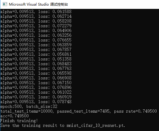
运行上述代码,得到的结果如下,可以看到对测试机分类的准确率达到了74.95%,相对于我们前文实现的Alexnet网络稍微有所提升,但是提升不多。
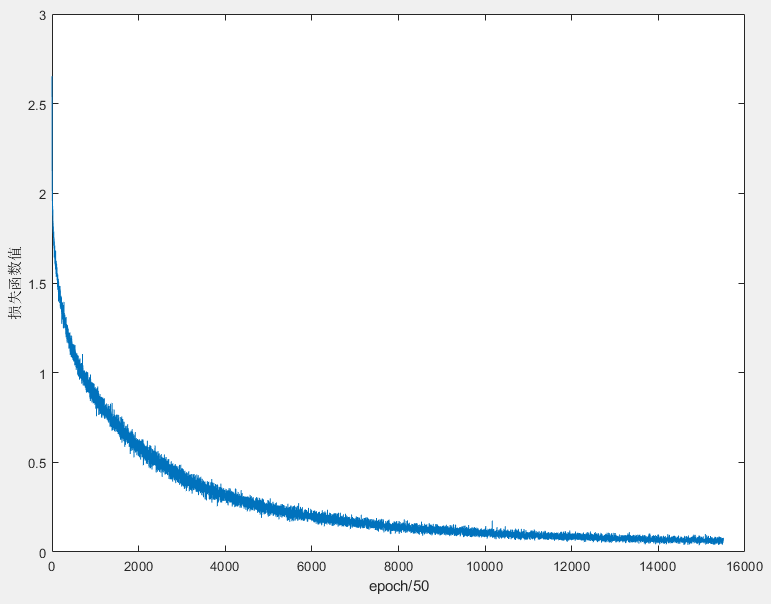
训练过程中损失函数值的变化过程如下图所示,可以看到损失函数值总体趋势是在下降的:
从自己实现简单的5层网络,到使用libtorch实现Lenet-5网络,接着到使用libtorch实现Alexnet网络,再到本文使用libtorch实现Resnet34网络,本来以为随着网络复杂度的提升,对Cifar-10分类的准确率也会有明显的提升,可是结果却并不是很理想,目前只是达到了74.95%,距离网络上大神们动不动90%以上的准确率还有点远。路漫漫其修远兮,吾将上下而求索,作为一个初学者,我会继续学习、探索,尝试调参、预处理、调整网络结构等手段来提高准确率,加油!
欢迎扫码关注本微信公众号,接下来会不定时更新更加精彩的内容,敬请期待~