Dijkstar-And-Astar算法

Dijkstra And A*

目录

• Dijkstra And A*
  • 1.0 引出
  • 2.0 Dijkstar Algorithm
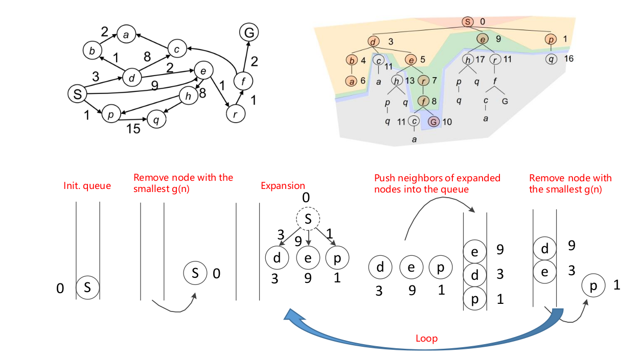
    • 2.1 整体流程
    • 2.2 算法伪代码
    • 2.3 Pros and Cons of Dijkstra’s Algorithm（优缺点）
  • 3.0 A* Algorithm
    • 3.1 启发式搜索 (Search Heuristic)
    • 3.2 A* ：Dijkstra with a Heuristic
    • 3.3 A* Optimality
      • 3.3.1 Admissible Heuristics
      • 3.3.2 Heuristic Design
    • 3.4 Dijkstra Vs A*
    • 3.5 Sub-optimal Solution

1.0 引出

$$ 首先，在一个实际上的最短路问题中，从图中一个节点到达另外一个邻居节点是有 Cost 这一说的，这个 Cost 可以是我们平常所说的 Length、Time、Energy. etc.

$$ 当所有的权重(Cost)都为 $1$ 的时候，BFS 将会找到最优解。所以对于一个通用的情况下，如何去找到一个最小代价的路径呢？这时 Dijkstar 算法便出场了。

2.0 Dijkstar Algorithm

$$ 其实 $Dijkstar$ 算法解决的是赋权图中最短路径规划问题，但是在日常的无人车的导航过程中，如果地图是基于普通的栅格地图，则每条路线的 $cost$ 都基本上要么是 $1$，要么是 $\sqrt{2}$ ，往往是比较简单的。

2.1 整体流程

$$$Dijkstra$ 弹出节点是根据当前节点中的一个累计 $cost$，找出最小的那个。简单来说其 Strategy is : expand/visit the node with cheapest accumulated cost $g(n)$。通常将其整个流程归结为以下三个步骤：

• g(n): The current best estimates of the accumulated cost from the start state to node “n”.
• Update the accumulated costs g(m) for all unexpanded neighbors “m” of node “n”.
• A node that has been expanded/visited is guaranteed to have the smallest cost from the start state.

$g(n)$ 表示的是从起点开始到当前节点的一个代价总和。

在弹出、扩展这两步的时候，弹出当前节点 $n$，然后找到当前节点的所有孩子节点并进行扩展，此时要计算当前节点 $g(n)$ 和每个孩子节点 $m$ 的一个代价值，及 $g(n)+m$ , 首先如果 $m$ 是没有被扩展过的节点，那么就会检测 g(m) 是否可以通过 $g(n)$ 进行下降，即把 $m$ 设置成从 $n$ 走到 $m$ ,看看是否新的代价 $g(m)$ 进行了下降，如果下降了则更新 $g(m)$。

$Dijkstar$ 算法是具有最优性质保证的，即保图中所有被扩展过的节点的 $cost$（从起点到当前节点的 $cost$）是最小的，这里不进行证明，设计具体的图论相关的知识，读者只需记住 $Dijkstar$ 算法是有完备的数学证明即可。

2.2 算法伪代码

$$下面通过伪代码对流程进行详细的解释。

• $Dijkstra$ 算法伪代码流程

• Mantain a priority queue to store all the nodes to be expanded。维护一个优先级队列去存储所有待扩展的节点。注意这里的优先级队列的意思，不同于之前我们在 BFS 时使用的简单队列，他对自动对当前队列中的元素进行排序，实际上在 C++ 实现的时候使用的是标准库中的 map，具体对应的是哈系表这一数据结构，学过的同学都知道他的查找效率是常数 $O(1)$。而我们在每次弹出的时候会自动弹出具有最小 g 值的节点。
• The priority queue is initialized with the start state $X_S$。优先级队列在初始化的时候只有一个起点 $X_S$。这里其他节点（除了起点）的代价值都初始化为了无穷大，是因为我们不知道从起点能否到达该节点，因此初始化为无穷大。
• Assign $g(X_S=0$) and $g(n)=infinite$ for all other nodes in the graph。对图中的所有初始节点进行赋值。
• Loop
  • if the queue is empty; return false; 如果优先级队列是空的，则算法结束，表示没找到节点，比如说是一个迷宫，或者是个死胡同。
  • Remove the node "n" with the lowest g(n) from the priority queue。从当前优先级队列中弹出 g 值最小的节点。对应了通用图搜索算法中的"弹出"。
  • Mark "n" as expanded。把 "n" 标记为已经扩展过的。throw the "n" into the close set。此时 "n" 已经不会再被扩展了。
  • if n is the goal node, return TRUE;break;
  • For all unexpanded neighbors "m" of node "n"
    • if g(m) = inifinite （说明这是一个仅仅在刚开始的时候初始化的节点，尚未被探索，则要对其进行操作）
      • g(m) = g(n) + Cnm(即边的代价)
      • Push node "m" into the queue(open set)将该节点添加到优先级队列中去，等待进行访问/扩展。
    • if g(m) > g(n) + Cnm （如果得到的新的路径的代价值小于当前的代价值，则需要更新该节点的代价值和父节点等相关信息。
      • g(m) g(n) + Cnm
  • end
• END LOOP

$$ 整体的一个流程如下图所示，形象的展示了从弹出到扩展的流程：

2.3 Pros and Cons of Dijkstra’s Algorithm（优缺点）

• The Good

  • Complete and optimal。完备并且是最优的，也就是说如果该问题有解，则 Dijkstar 算法一定能找到并且是最优的。

• The Bad

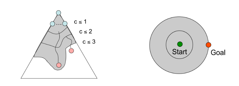
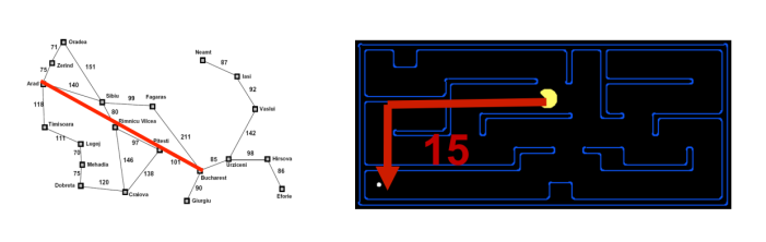
  • Can only see the cost accumulated so far (i.e. the uniform cost), thus exploring next state in every “direction”。

  • No information about goal location。

  • 上述两个缺点体现在如下这张图上

    

$$ 上述缺点明显是能够通过某种方式解决的，还记得上一篇文章介绍过的贪心搜索，充分利用了起点和目标点的一个信心进行路径的扩展和搜索，是否可以将贪心搜索融入到 Dijkstar 算法中去呢？答案是可以的，结合 heuristic search 之后，Dijkstar 算法便成为了我们所熟知的 A* 算法。

3.0 A* Algorithm

3.1 启发式搜索 (Search Heuristic)

$$ 其实前面介绍的贪心搜索就是启发式搜索的一种。通过推断距离目标的最小成本来克服距离每个点都是一样的成本搜索的缺点（例如使用距离目标点的距离函数等）。而对于特定的问题则应该设定不同的一个启发函数，例如欧式距离隐式认为机器人可以朝着对角线的方向移动，但是事实上很多机器人并不是这样的，有的只能平移，有的则要根据前轮的一个角度才能进行转向，也就是自行车模型或者阿克曼转向模型等。因此，对于具体的机器人，要设计不同的一个启发式函数。

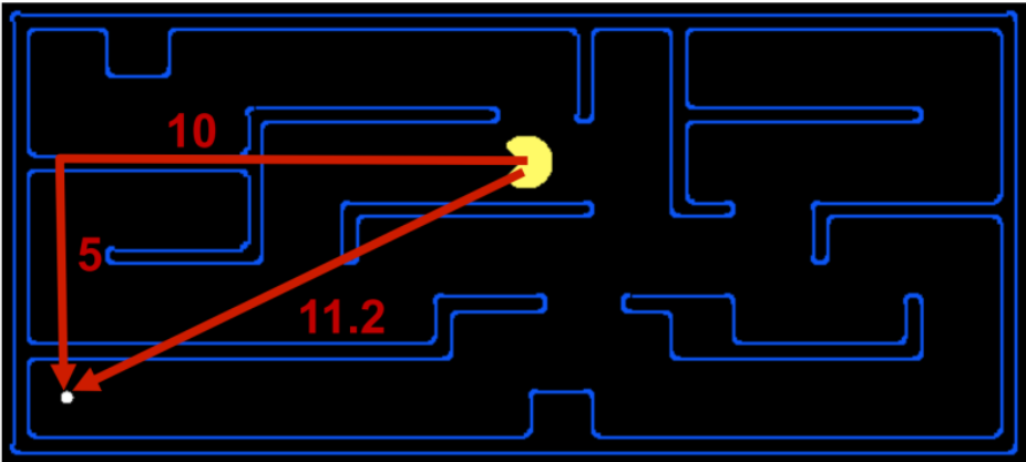
$$ 我们在前面已经提到的启发函数，例如 Manhattan Distance VS. Euclidean Distance

3.2 A* ：Dijkstra with a Heuristic

$$ 其实，本质上 A* 就是 Dijkstar 算法基础上加入了 Heuristic Function，使用了启发是搜索，进而整体上加快了搜索速度，或者说是加快了朝目标点搜索的速度。下面我们来看一下 A* 算法中比较重要的几个点：

• Accumulated cost （累计代价）
  • g(n): The current best estimate of the accumulated cost from the start to end node "n"。从起始状态到节点“n”的累积成本的当前最佳估计。
• Heuristic
  • h(n) : The estimated least cost from node n to goal state (i.e. goal cost)。从节点 n 到目标状态的估计最小成本（即目标成本）。
• The least estimated cost from start state to goal state passing through node “n” is f(n) = g(n) + h(n)。通过节点“n”从起始状态到目标状态的最小估计成本为 f(n) = g(n) + h(n)
• Strategy: expand the node with cheapest f(n) = g(n) + h(n)。策略：扩展最便宜的节点 f(n) = g(n) + h(n)。
  • Update the accumulated costs g(m) for all unexpanded neighbors “m” of node “n”。更新节点“n”的所有未扩展邻居“m”的累积成本 g(m)
  • A node that has been expanded is guaranteed to have the smallest cost from the start state。已扩展的节点保证从开始状态具有最小的成本。

A Algorithm Wokrflow*

• Mantain a priority queue to store all the nodes to be expanded。维护一个优先级队列去存储所有待扩展的节点。注意这里的优先级队列的意思，不同于之前我们在 BFS 时使用的简单队列，他对自动对当前队列中的元素进行排序，实际上在 C++ 实现的时候使用的是标准库中的 map，具体对应的是哈系表这一数据结构，学过的同学都知道他的查找效率是常数 $O(1)$。而我们在每次弹出的时候会自动弹出具有最小 g 值的节点。
• The priority queue is initialized with the start state $X_S$。优先级队列在初始化的时候只有一个起点 $X_S$。这里其他节点（除了起点）的代价值都初始化为了无穷大，是因为我们不知道从起点能否到达该节点，因此初始化为无穷大。
• Assign $g(X_S=0$) and $g(n)=infinite$ for all other nodes in the graph。对图中的所有初始节点进行赋值。
• Loop
• if the queue is empty; return false; 如果优先级队列是空的，则算法结束，表示没找到节点，比如说是一个迷宫，或者是个死胡同。
• Remove the node "n" with the lowest g(n) from the priority queue。从当前优先级队列中弹出 g 值最小的节点。对应了通用图搜索算法中的"弹出"。
• Mark "n" as expanded。把 "n" 标记为已经扩展过的。throw the "n" into the close set。此时 "n" 已经不会再被扩展了。
• if n is the goal node, return TRUE;break;
• For all unexpanded neighbors "m" of node "n"
  • if g(m) = inifinite （说明这是一个仅仅在刚开始的时候初始化的节点，尚未被探索，则要对其进行操作）
    • g(m) = g(n) + Cnm(即边的代价)
    • Push node "m" into the queue(open set)将该节点添加到优先级队列中去，等待进行访问/扩展。
  • if g(m) > g(n) + Cnm （如果得到的新的路径的代价值小于当前的代价值，则需要更新该节点的代价值和父节点等相关信息。
    • g(m) g(n) + Cnm
• end
• END LOOP

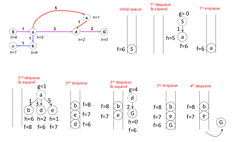
这里也给出一个 A* 算法的整体流程，如下图所示：

$$ 与 Dijkstra 算法不同的是，在每次计算 cost 的时候，分成了两个部分，分别是边的权重（通常是距离）和 Heuristic Cost。其他部分则和 Dijkstra 算法并无太大区别。

3.3 A* Optimality

$$ 但是，加入 Heuristic Function 后，如果 Heuristic Function 设计不当就会打破 Dijkstra 算法原有的最优性的保证，如下图所示：

$$ 首先说明一点，从节点 S 到节点 G 的最优路径我们一眼即可看出是先经过 A 点，然后到达 G 点，这才是最优路径，但是当加入了 Heuristic 之后，我们再使用 A* 来计算一下。

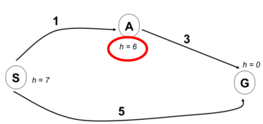
• 首先弹出节点 S
• 将 A 和 G 入队，保存到 A 和 G 的 cost 和 Heuristic。
• 计算得到 $f_A=1+6=7$。$f_G=5+0$ 。
• 发现 $f_G<f_A$ 则弹出 G，并判断 G 是否是目标点
• 是则结束搜索。
• 最终得到的最短路径是 $S\to G$

$$ 很明显，这并不是最优解，为什么呢，试想一下本身 Dijkstra 算法是能够保证找到的路径是最优解的，但是在加入 Heuristic Function 之后发现却不可以了，很明显是 Heuristic Function 不合理导致的，那么什么样的 Heuristic Function 才是能够真正使用的呢？

• The answer is:

  启发式函数所估计出的 cost 要至少是小于等于真正的 cost。而是否真正的合理有的时候还要根据机器人的一个运动学模型来进行选择，例如对于全向轮机器人来说，欧式距离是可以的，但是曼哈顿距离则不行。上面那个例子中 A 点的 H 为 6，明显大于真实机器人距离目标点的 cost。

3.3.1 Admissible Heuristics

• 一个可以接受并进行使用的 Heuristic $H(\cdot )$ 需要满足如下条件（和上面说的一样）

  对于所有的节点来说：$h(n)<=h^{\ast }(n)$ ，其中 $h^{\ast }(n)$ 是所有节点 n 到达目标点的真实最短距离。

• 如果 heuristic 是 admissible，那么 A* 搜索算法得到的结果一定是最优的。

• 提出 Admissible Heuristics 是在实践中使用 A* 最为重要核心的部分。

• 下面是两种不同 Heuristic

3.3.2 Heuristic Design

$$ Admissible Heuristic Function 需要根据特定的使用场景和机器人模型 design case by case。

• Is Euclidean distance (L2 norm) admissible? Yes

• Is Manhattan distance (L1 norm) admissible? Depends

• Is L∞ norm distance admissible? Yes

• Is 0 distance admissible? Always

3.4 Dijkstra Vs A*

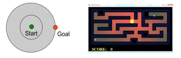
• Dijkstra 算法朝着所有的方向进行扩展，不带目的性。如下图所示：

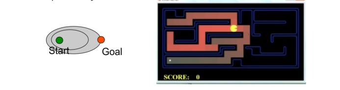
• A* 则带有目的性的进行扩展，如下图所示：

3.5 Sub-optimal Solution

$$ 当我们使用了一个过估计的 heuristic function 之后会出现什么效果呢？很明显，上面看到的圆形会更加的椭，但是控制好这个度。这样是能够明显提高我们的一个搜索速度的，但是也要承担相应的风险，因为这样并不能够保证求得的解是最优解。例如 Weighted A* 算法。

$$ 可以看到和 A* 的区别在于 $f$ 函数的不同，此时在 Heuristic 前加上了一个系数变成了 $\mathrm{f}=\mathrm{g}+\epsilon \mathrm{h},\epsilon >1$。

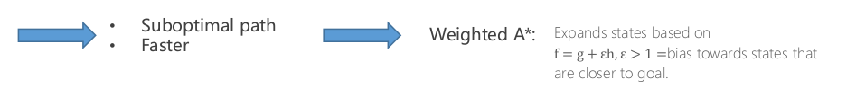
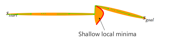
• Weighted A Search:*
  • 在最优和速度之间进行折中
  • $\epsilon$-suboptimal: cost(solution) <= $\epsilon$cost(optimal solution)
  • 它可以比 A* 快几个数量级