第七章习题

学号后四位:3018
7.3:

点击查看代码

import numpy as np
import matplotlib.pyplot as plt
from scipy.interpolate import interp1d, CubicSpline

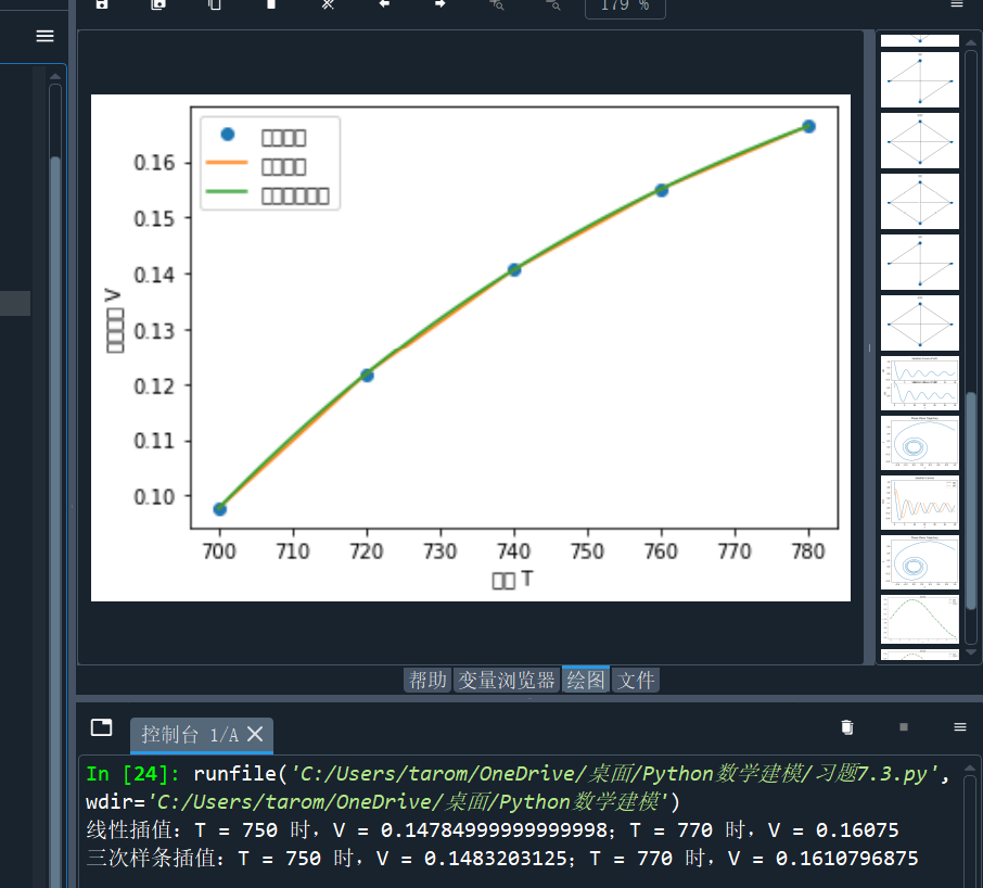
T = np.array([700, 720, 740, 760, 780])
V = np.array([0.0977, 0.1218, 0.1406, 0.1551, 0.1664])

# 线性插值
linear_interp = interp1d(T, V)
V_linear_750 = linear_interp(750)
V_linear_770 = linear_interp(770)

# 三次样条插值
cubic_interp = CubicSpline(T, V)
V_cubic_750 = cubic_interp(750)
V_cubic_770 = cubic_interp(770)

print(f"线性插值：T = 750 时，V = {V_linear_750}；T = 770 时，V = {V_linear_770}")
print(f"三次样条插值：T = 750 时，V = {V_cubic_750}；T = 770 时，V = {V_cubic_770}")

# 绘制图形
T_new = np.linspace(700, 780, 100)
V_linear_new = linear_interp(T_new)
V_cubic_new = cubic_interp(T_new)

plt.plot(T, V, 'o', label='原始数据')
plt.plot(T_new, V_linear_new, label='线性插值')
plt.plot(T_new, V_cubic_new, label='三次样条插值')
plt.xlabel('温度 T')
plt.ylabel('体积变化 V')
plt.legend()
plt.show()
print("xuehao3018")

7.4:

点击查看代码

import numpy as np
import matplotlib.pyplot as plt
from scipy.interpolate import griddata

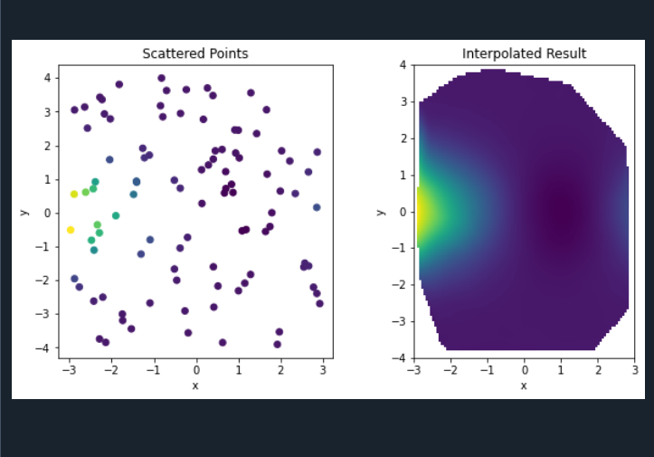
# 定义函数
def f(x, y):
    return (x**2 - 2*x) * np.exp(-y**2/2)

# 生成随机散乱点
np.random.seed(0)
n_points = 100
x_random = np.random.uniform(-3, 3, n_points)
y_random = np.random.uniform(-4, 4, n_points)
z_random = f(x_random, y_random)

# 定义插值网格
grid_x, grid_y = np.mgrid[-3:3:100j, -4:4:100j]

# 进行插值
z_interpolated = griddata((x_random, y_random), z_random, (grid_x, grid_y), method='cubic')

# 绘制结果
plt.figure(figsize=(10, 5))
plt.subplot(121)
plt.scatter(x_random, y_random, c=z_random, cmap='viridis')
plt.title('Scattered Points')
plt.xlabel('x')
plt.ylabel('y')

plt.subplot(122)
plt.imshow(z_interpolated.T, extent=[-3, 3, -4, 4], origin='lower', cmap='viridis')
plt.title('Interpolated Result')
plt.xlabel('x')
plt.ylabel('y')

plt.show()
print("xuehao3018")

7.7：

点击查看代码

import numpy as np
from scipy.optimize import curve_fit, least_squares
import matplotlib.pyplot as plt

# 定义函数 g(x)
def g(x, j0, q, r):
    return j0 * (1.1 ** x) + (q - 1.1 * j0) * r * x

# 生成模拟观测值
a = 1.1
b = 0.01
x_data = np.arange(1, 21)
y_data = [g(x, a, a + b, b) for x in x_data]

# 1. 用 curve_fit 拟合函数 g(x)
popt_curve_fit, _ = curve_fit(g, x_data, y_data)
y_curve_fit = g(x_data, *popt_curve_fit)

# 2. 用 leastsq 拟合函数 g(x)（注意：leastsq 在较新版本的 scipy 中已被弃用，这里只是为了演示）
from scipy.optimize import leastsq

def residuals(params, x, y):
    return y - g(x, *params)

initial_guess = [1, 1, 1]
popt_leastsq, _ = leastsq(residuals, initial_guess, args=(x_data, y_data))
y_leastsq = g(x_data, *popt_leastsq)

# 3. 用 least_squares 拟合函数 g(x)
def fun(params):
    return g(x_data, *params) - y_data

initial_guess_ls = [1, 1, 1]
res_ls = least_squares(fun, initial_guess_ls)
popt_least_squares = res_ls.x
y_least_squares = g(x_data, *popt_least_squares)

# 绘制结果
plt.plot(x_data, y_data, 'o', label='模拟观测值')
plt.plot(x_data, y_curve_fit, label='curve_fit')
plt.plot(x_data, y_leastsq, label='leastsq')
plt.plot(x_data, y_least_squares, label='least_squares')
plt.legend()
plt.xlabel('x')
plt.ylabel('g(x)')
plt.show()
print("xuehao3018")

7.10:

点击查看代码

import numpy as np
import matplotlib.pyplot as plt
from scipy.interpolate import interp1d
from scipy.optimize import curve_fit

# 数据
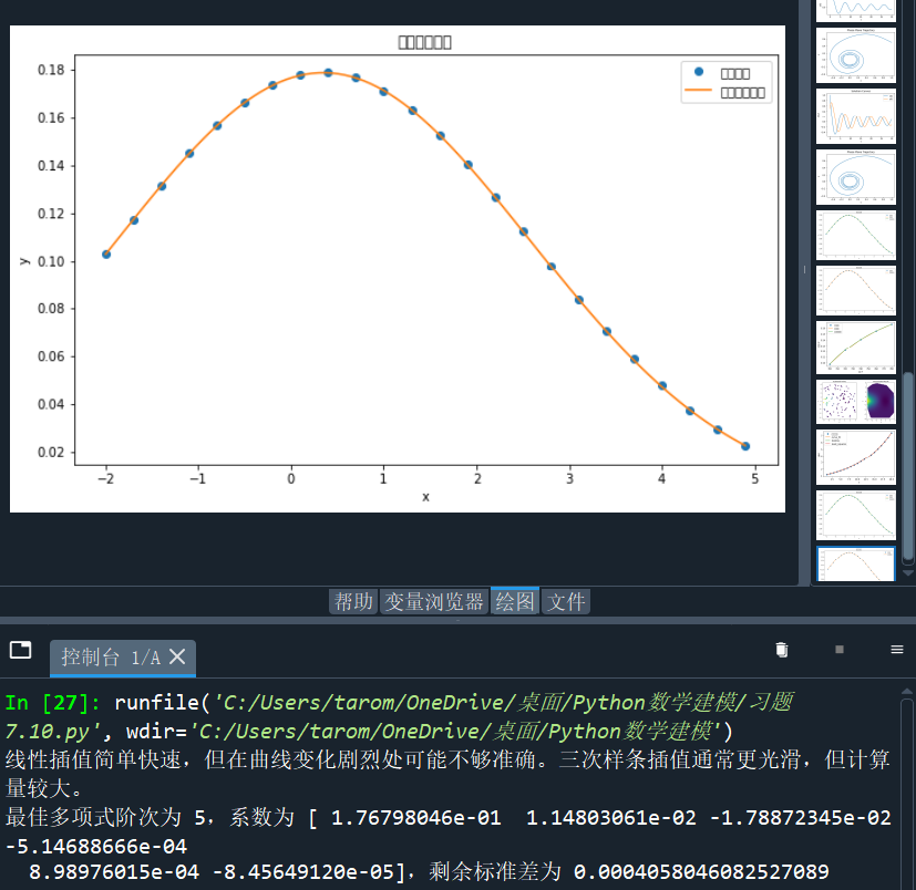
x_data = np.array([-2, -1.7, -1.4, -1.1, -0.8, -0.5, -0.2, 0.1, 0.4, 0.7, 1, 1.3, 1.6, 1.9, 2.2, 2.5, 2.8, 3.1, 3.4, 3.7, 4, 4.3, 4.6, 4.9])
y_data = np.array([0.1029, 0.1174, 0.1316, 0.1448, 0.1566, 0.1662, 0.1733, 0.1775, 0.1785, 0.1764, 0.1711, 0.1630, 0.1526, 0.1402, 0.1266, 0.1122, 0.0977, 0.0835, 0.0702, 0.0588, 0.0479, 0.0373, 0.0291, 0.0224])

# 1. 插值方法绘制曲线并比较
# 线性插值
linear_interp = interp1d(x_data, y_data, kind='linear')
x_linear = np.linspace(-2, 4.9, 100)
y_linear = linear_interp(x_linear)

# 三次样条插值
cubic_interp = interp1d(x_data, y_data, kind='cubic')
x_cubic = np.linspace(-2, 4.9, 100)
y_cubic = cubic_interp(x_cubic)

# 绘制插值结果
plt.figure(figsize=(10, 6))
plt.plot(x_data, y_data, 'o', label='原始数据')
plt.plot(x_linear, y_linear, label='线性插值')
plt.plot(x_cubic, y_cubic, label='三次样条插值')
plt.xlabel('x')
plt.ylabel('y')
plt.title('插值方法比较')
plt.legend()

# 比较优劣（简单描述）
print("线性插值简单快速，但在曲线变化剧烈处可能不够准确。三次样条插值通常更光滑，但计算量较大。")

# 2. 多项式拟合
def polynomial_func(x, *coeffs):
    y = 0
    for i, c in enumerate(coeffs):
        y += c * x**i
    return y

degrees = [2, 3, 4, 5]
best_degree = None
best_residuals = None
best_coeffs = None

for degree in degrees:
    initial_coeffs = np.ones(degree + 1)
    popt, _ = curve_fit(polynomial_func, x_data, y_data, p0=initial_coeffs)
    residuals = y_data - polynomial_func(x_data, *popt)
    if best_residuals is None or np.sum(residuals**2) < best_residuals:
        best_degree = degree
        best_residuals = np.sum(residuals**2)
        best_coeffs = popt

print(f"最佳多项式阶次为 {best_degree}，系数为 {best_coeffs}，剩余标准差为 {np.sqrt(best_residuals / len(x_data))}")

# 3. 正态分布拟合
def normal_dist_func(x, mu, sigma):
    return 1 / (sigma * np.sqrt(2 * np.pi)) * np.exp(-(x - mu)**2 / (2 * sigma**2))

popt_normal, _ = curve_fit(normal_dist_func, x_data, y_data)
mu_fit, sigma_fit = popt_normal

x_normal = np.linspace(-2, 4.9, 100)
y_normal = normal_dist_func(x_normal, mu_fit, sigma_fit)

plt.figure(figsize=(10, 6))
plt.plot(x_data, y_data, 'o', label='原始数据')
plt.plot(x_normal, y_normal, label='正态分布拟合')
plt.xlabel('x')
plt.ylabel('y')
plt.title('正态分布拟合')
plt.legend()

plt.show()
print("xuehao3018")