岭回归、Lasso回归、logistic回归模型、决策树、随机森林与K近邻模型

模型的假设检验（F与T）

F检验

提出原假设和备用假设，之后计算统计量与理论值，最后进行比较。

F校验主要检验的是模型是否合理。

导入第三方模块

import numpy as np
import pandas as pd
from sklearn import model_selection
import statsmodels.api as sm

# 数据处理
Profit = pd.read_excel(r'Predict to Profit.xlsx')
dummies = pd.get_dummies(Profit.State)
Profit_New = pd.concat([Profit,dummies], axis = 1)
Profit_New.drop(labels = ['State','New York'], axis = 1, inplace = True) 
train, test = model_selection.train_test_split(Profit_New, test_size = 0.2, random_state=1234)
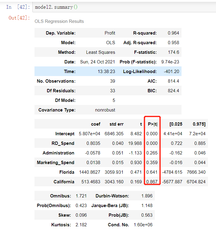
model2 = sm.formula.ols('Profit~RD_Spend+Administration+Marketing_Spend+Florida+California', data = train).fit()

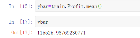
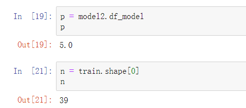
统计变量个和观测个数

ybar=train.Profit.mean()

统计变量个数和观察个数

p=model2.df_model
n=train.shape[0]

计算回归离差平方和

RSS=np.sum((model2.fittedvalues-ybar)**2)

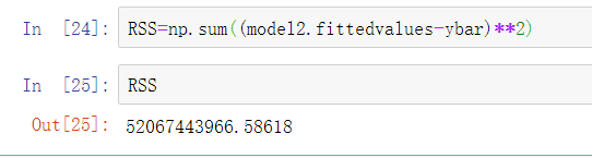
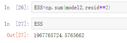
计算误差平方和

ESS=np.sum(model2.resid**2)

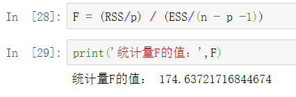
计算F统计量的值

F=(RSS/p)/(ESS/(n-p-1))
print('F统计量的值：',F)

计算F分布的理论值

from scipy.stats import f
# 计算F分布的理论值
F_Theroy = f.ppf(q=0.95, dfn = p,dfd = n-p-1)
print('F分布的理论值为：',F_Theroy)

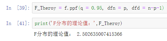
结论：

可以看到计算出来的F统计值（174.6）远远大于F分布的理论值（2.5），所以应该拒绝原假设。

T检验

T检验更加侧重于检验模型的各个参数是否合理。

model.summary()  # 绝对值越小影响越大

线性回归模型的短板

自变量的个数大于样本量

自变量之间存在多重共线性

解决线性回归模型的短板

岭回归模型

在线性回归模型的基础之上添加一个l2惩罚项(平方项、正则项)，该模型最终转变成求解圆柱体与椭圆抛物线的焦点问题。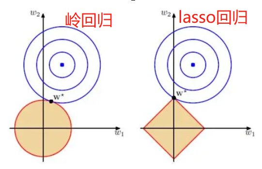

Lasso回归模型

在线性回归模型的基础之上添加一个l1惩罚项(绝对值项、正则项)

相较于岭回归降低了模型的复杂度，该模型最终转变成求解正方体与椭圆抛物线的焦点问题。

交叉验证

将所有数据都参与到模型的构建和测试中最后生成多个模型，再从多个模型中筛选出得分最高(准确度)的模型。

岭回归模型的交叉验证

数据准备

# 导入第三方模块
import pandas as pd
import numpy as np
from sklearn import model_selection
from sklearn.linear_model import Ridge,RidgeCV
import matplotlib.pyplot as plt

# 读取糖尿病数据集
diabetes = pd.read_excel(r'diabetes.xlsx', sep = '')
# 构造自变量（剔除患者性别、年龄和因变量）
predictors = diabetes.columns[2:-1]
# 将数据集拆分为训练集和测试集
X_train, X_test, y_train, y_test = model_selection.train_test_split(diabetes[predictors], diabetes['Y'], 
                                                                    test_size = 0.2, random_state = 1234 )

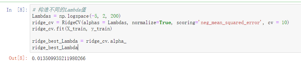
获得lambda数值

# 构造不同的Lambda值
Lambdas = np.logspace(-5, 2, 200)
# 岭回归模型的交叉验证
# 设置交叉验证的参数，对于每一个Lambda值，都执行10重交叉验证
ridge_cv = RidgeCV(alphas = Lambdas, normalize=True, scoring='neg_mean_squared_error', cv = 10)
# 模型拟合
ridge_cv.fit(X_train, y_train)
# 返回最佳的lambda值
ridge_best_Lambda = ridge_cv.alpha_
ridge_best_Lambda

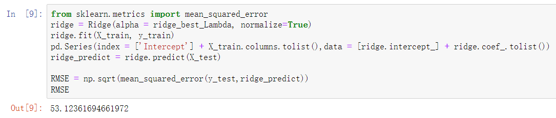
预测

# 导入第三方包中的函数
from sklearn.metrics import mean_squared_error
# 基于最佳的Lambda值建模
ridge = Ridge(alpha = ridge_best_Lambda, normalize=True)
ridge.fit(X_train, y_train)
# 返回岭回归系数
pd.Series(index = ['Intercept'] + X_train.columns.tolist(),data = [ridge.intercept_] + ridge.coef_.tolist())
# 预测
ridge_predict = ridge.predict(X_test)
# 预测效果验证
RMSE = np.sqrt(mean_squared_error(y_test,ridge_predict))
RMSE

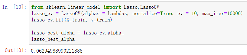
lasso回归模型交叉验证

获取lambda值

# 导入第三方模块中的函数
from sklearn.linear_model import Lasso,LassoCV
# LASSO回归模型的交叉验证
lasso_cv = LassoCV(alphas = Lambdas, normalize=True, cv = 10, max_iter=10000)
lasso_cv.fit(X_train, y_train)
# 输出最佳的lambda值
lasso_best_alpha = lasso_cv.alpha_
lasso_best_alpha

建模并预测

# 基于最佳的lambda值建模
lasso = Lasso(alpha = lasso_best_alpha, normalize=True, max_iter=10000)
lasso.fit(X_train, y_train)
# 返回LASSO回归的系数
pd.Series(index = ['Intercept'] + X_train.columns.tolist(),data = [lasso.intercept_] + lasso.coef_.tolist())

# 预测
lasso_predict = lasso.predict(X_test)
# 预测效果验证
RMSE = np.sqrt(mean_squared_error(y_test,lasso_predict))
RMSE

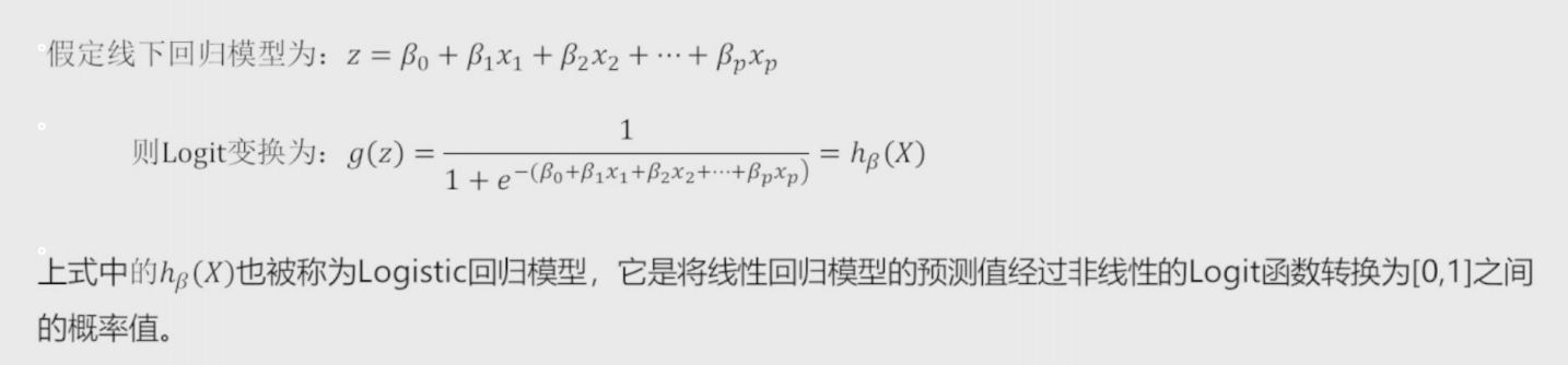
Logistic回归模型

将线性回归模型的公式做Logit变换，即为Logistic回归模型，将预测问题变成了0到1之间的概率问题。

混淆矩阵

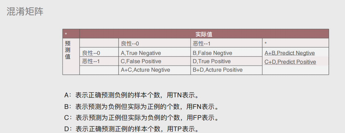
准确率

表示正确预测的正负例样本数与所有样本数量的⽐值，即(A+D)/(A+B+C+D)

正例覆盖率

表示正确预测的正例数在实际正例数中的⽐例，即D/(B+D)

负例覆盖率

表示正确预测的负例数在实际负例数中的⽐例，即A/(A+C)

正例命中率

表示正确预测的正例数在预测正例数中的⽐例，即D/(C+D)

代码

# 导入第三方模块
import pandas as pd
import numpy as np
from sklearn import model_selection
from sklearn import linear_model

# 读取数据
sports = pd.read_csv(r'Run or Walk.csv')
# 提取出所有自变量名称
predictors = sports.columns[4:]
# 构建自变量矩阵
X = sports.ix[:,predictors]
# 提取y变量值
y = sports.activity
# 将数据集拆分为训练集和测试集
X_train, X_test, y_train, y_test = model_selection.train_test_split(X, y, test_size = 0.25, random_state = 1234)

# 利用训练集建模
sklearn_logistic = linear_model.LogisticRegression()
sklearn_logistic.fit(X_train, y_train)
# 返回模型的各个参数
print(sklearn_logistic.intercept_, sklearn_logistic.coef_)
# 模型预测
sklearn_predict = sklearn_logistic.predict(X_test)
# 预测结果统计
pd.Series(sklearn_predict).value_counts()

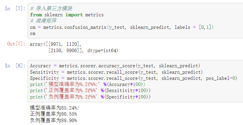
# 导入第三方模块
from sklearn import metrics
# 混淆矩阵
cm = metrics.confusion_matrix(y_test, sklearn_predict, labels = [0,1])
cm

Accuracy = metrics.scorer.accuracy_score(y_test, sklearn_predict)
Sensitivity = metrics.scorer.recall_score(y_test, sklearn_predict)
Specificity = metrics.scorer.recall_score(y_test, sklearn_predict, pos_label=0)
print('模型准确率为%.2f%%:' %(Accuracy*100))
print('正例覆盖率为%.2f%%' %(Sensitivity*100))
print('负例覆盖率为%.2f%%' %(Specificity*100))

模型的评估方法

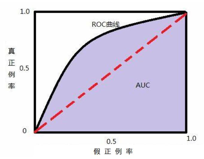
ROC曲线

通过计算AUC阴影部分的面积来判断模型是否合理（通常大于0.8表示合理）

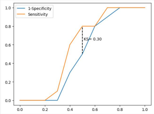
KS曲线

通过计算两条折线之间最大距离来衡量模型是否合理（通常大于0.4表示合理）

绘制KS曲线代码

def内的代码保存下来即可

# 导入第三方模块
import pandas as pd
import numpy as np
import matplotlib.pyplot as plt

# 自定义绘制ks曲线的函数
def plot_ks(y_test, y_score, positive_flag):
    # 对y_test重新设置索引
    y_test.index = np.arange(len(y_test))
    # 构建目标数据集
    target_data = pd.DataFrame({'y_test':y_test, 'y_score':y_score})
    # 按y_score降序排列
    target_data.sort_values(by = 'y_score', ascending = False, inplace = True)
    # 自定义分位点
    cuts = np.arange(0.1,1,0.1)
    # 计算各分位点对应的Score值
    index = len(target_data.y_score)*cuts
    scores = np.array(target_data.y_score)[index.astype('int')]
    # 根据不同的Score值，计算Sensitivity和Specificity
    Sensitivity = []
    Specificity = []
    for score in scores:
        # 正例覆盖样本数量与实际正例样本量
        positive_recall = target_data.loc[(target_data.y_test == positive_flag) & (target_data.y_score>score),:].shape[0]
        positive = sum(target_data.y_test == positive_flag)
        # 负例覆盖样本数量与实际负例样本量
        negative_recall = target_data.loc[(target_data.y_test != positive_flag) & (target_data.y_score<=score),:].shape[0]
        negative = sum(target_data.y_test != positive_flag)
        Sensitivity.append(positive_recall/positive)
        Specificity.append(negative_recall/negative)
    # 构建绘图数据
    plot_data = pd.DataFrame({'cuts':cuts,'y1':1-np.array(Specificity),'y2':np.array(Sensitivity), 
                              'ks':np.array(Sensitivity)-(1-np.array(Specificity))})
    # 寻找Sensitivity和1-Specificity之差的最大值索引
    max_ks_index = np.argmax(plot_data.ks)
    plt.plot([0]+cuts.tolist()+[1], [0]+plot_data.y1.tolist()+[1], label = '1-Specificity')
    plt.plot([0]+cuts.tolist()+[1], [0]+plot_data.y2.tolist()+[1], label = 'Sensitivity')
    # 添加参考线
    plt.vlines(plot_data.cuts[max_ks_index], ymin = plot_data.y1[max_ks_index], 
               ymax = plot_data.y2[max_ks_index], linestyles = '--')
    # 添加文本信息
    plt.text(x = plot_data.cuts[max_ks_index]+0.01,
             y = plot_data.y1[max_ks_index]+plot_data.ks[max_ks_index]/2,
             s = 'KS= %.2f' %plot_data.ks[max_ks_index])
    # 显示图例
    plt.legend()
    # 显示图形
    plt.show()

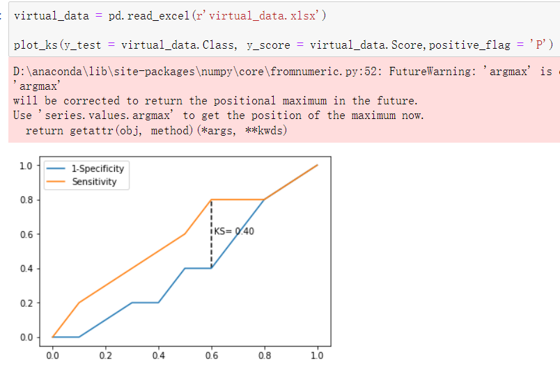
# 应用自定义函数绘制k-s曲线
virtual_data = pd.read_excel(r'virtual_data.xlsx')
plot_ks(y_test = virtual_data.Class, y_score = virtual_data.Score,positive_flag = 'P')

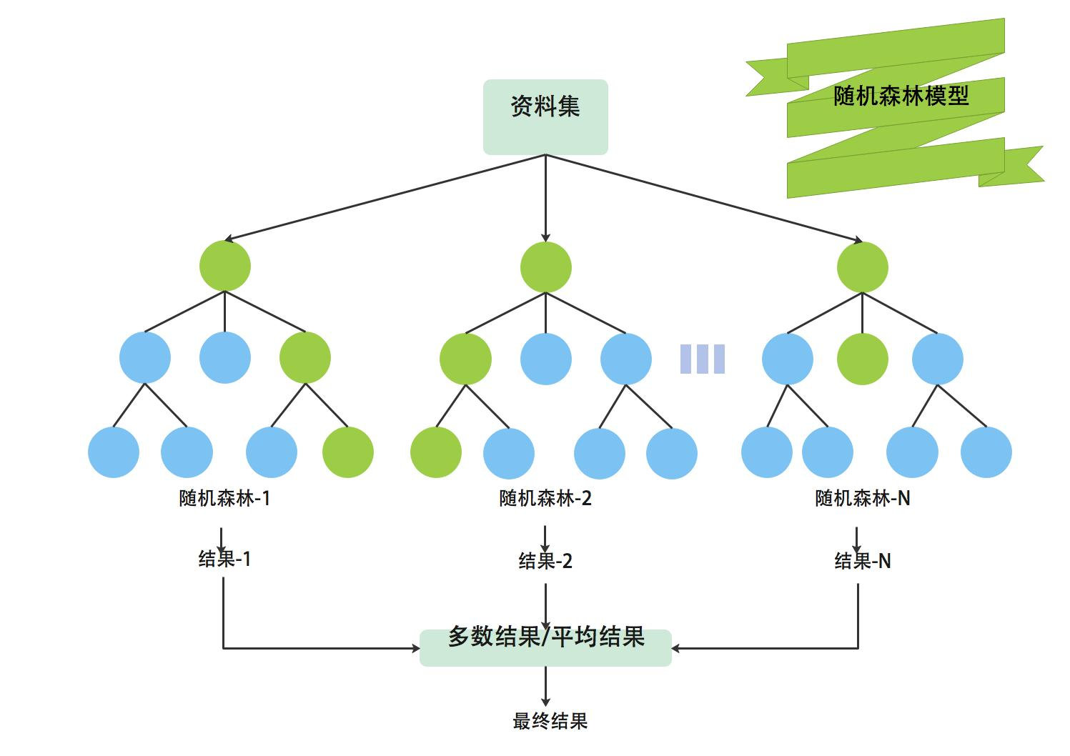
决策树与随机森林

默认情况下解决分类问题（买与不买，带与不带，走与不走），也可以切换算法解决预测问题（具体数值）

决策树

树其实是一种计算机底层的数据结构，计算机里的书都是自上而下的生长。

决策树则是算法模型中的一种概念有三个主要部分

根节点、枝节点

用于存放条件

叶子节点

存放真正的数据结果

信息熵

信息熵小的时候相当于红绿灯情况

信息熵大的时候相当于买彩票中奖情况

条件熵

由信息熵再次细分获得

例如：有九个用户购买了商品，五个用户没有购买，那么条件熵就是继续从购买或者不购买的用户中再选择一个条件进行判断：比如按照性别计算男和女的熵

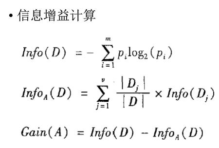
信息增益

信息增益可以反映出某个条件是否对最终的分类有决定性的影响。

在特征选择的时候常常用信息增益，构建决策树时根节点与枝节点所放的条件按照信息增益由大到小排，如果信息增益大的话，那么这个特征对于分类来说很关键。

信息增益率

决策树中的ID3算法使⽤信息增益指标实现根节点或中间节点的字段选择，但是该指标存在⼀个⾮常明显的缺点，即信息增益会偏向于取值较多的字段。

为了克服信息增益指标的缺点，提出了信息增益率的概念，它的思想很简单，就是在信息增益的基础上进⾏相应的惩罚。

基尼指数

可以让模型解决预测问题。

基尼指数增益

与信息增益类似，还需要考虑⾃变量对因变量的影响程度，即因变量的基尼指数下降速度的快慢，下降得越快，⾃变量对因变量的影响就越强。

随机森林

随机森林中每颗决策树都不限制节点字段选择，有多棵树组成的随机森林

在解决分类问题的时候采用投票法（多数结果）、解决预测问题的时候采用均值法（平均结果）

K近邻模型

思想：根据位置样本点周边k个邻居样本完成预测或者分类。

K值的选择

先猜测

交叉验证

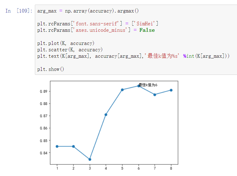
作图选择最合理的K值

过拟合与欠拟合

过拟合

训练误差和测试误差之间的差距太大，也就是模型复杂度高于实际问题，模型在训练集上表现很好，但在测试集上却表现很差。

欠拟合

模型不能在训练集上获得足够低的误差，换句话说，就是模型复杂度低，模型在训练集上就表现很差。

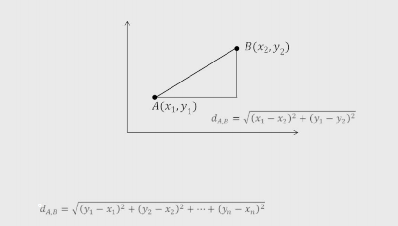
距离

欧氏距离

两点间的直线距离。

曼哈顿距离

就像走路需要的实际距离

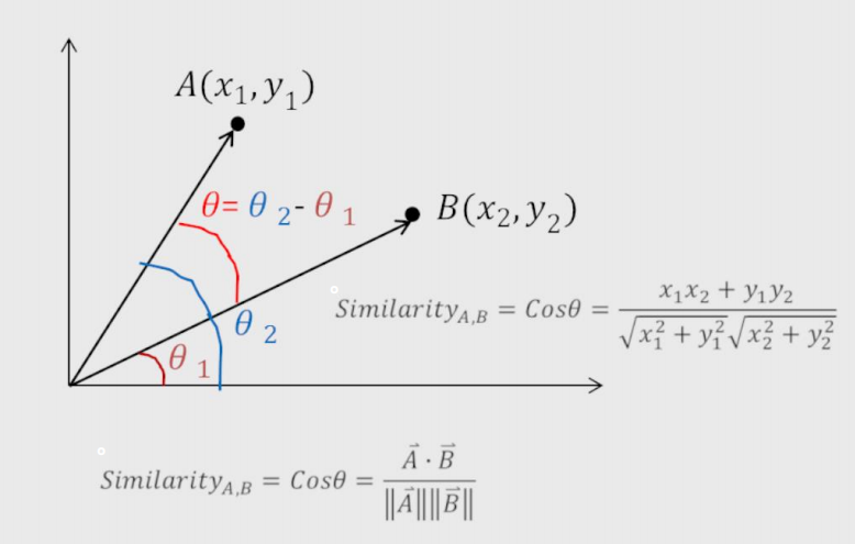
余弦相似度

查重时使用

K值计算代码演示

import numpy as np
import pandas as pd
from sklearn import model_selection
import matplotlib.pyplot as plt
from sklearn import neighbors

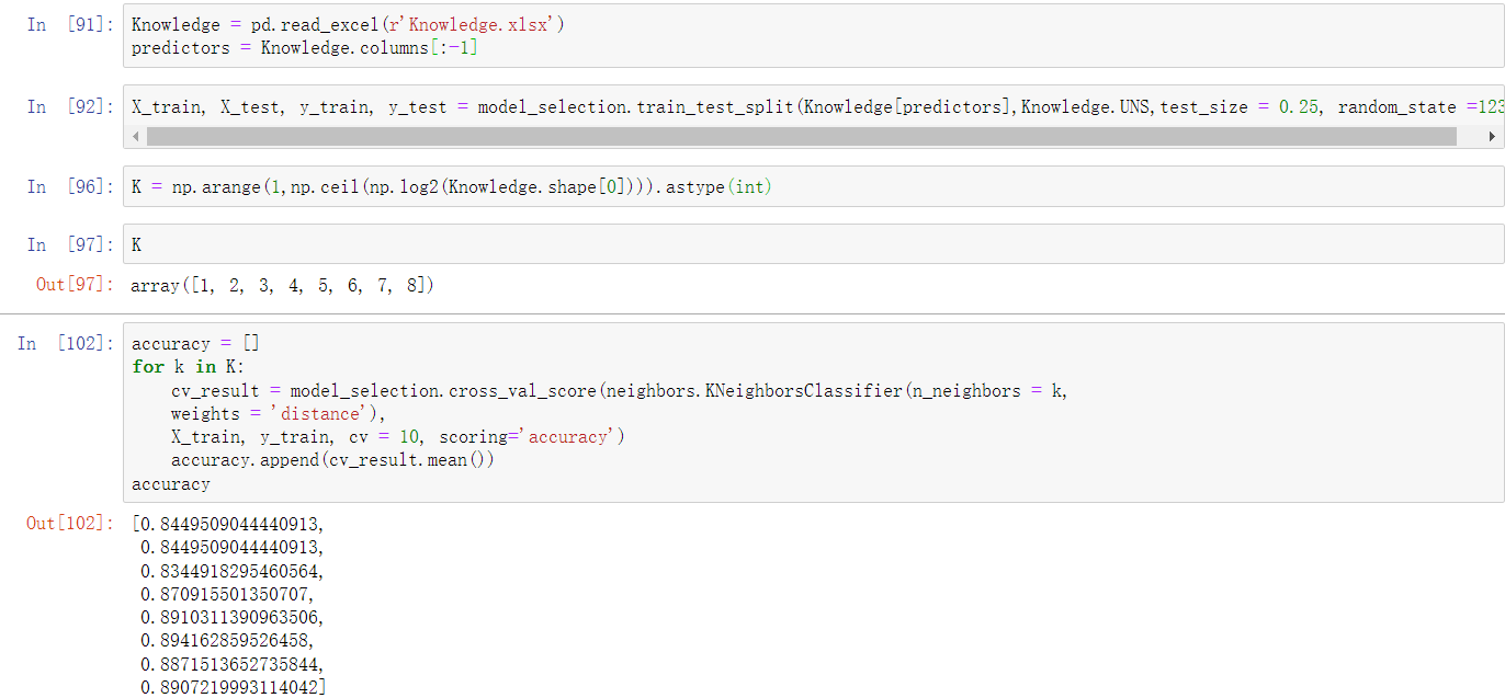
Knowledge = pd.read_excel(r'Knowledge.xlsx')
predictors = Knowledge.columns[:-1]
X_train, X_test, y_train, y_test = model_selection.train_test_split(Knowledge[predictors],Knowledge.UNS,test_size = 0.25, random_state =1234)
K = np.arange(1,np.ceil(np.log2(Knowledge.shape[0]))).astype(int)
accuracy = []
for k in K:
    cv_result = model_selection.cross_val_score(neighbors.KNeighborsClassifier(n_neighbors = k,
    weights = 'distance'),
    X_train, y_train, cv = 10, scoring='accuracy')
    accuracy.append(cv_result.mean())
arg_max = np.array(accuracy).argmax()

plt.rcParams['font.sans-serif'] = ['SimHei']
plt.rcParams['axes.unicode_minus'] = False

plt.plot(K, accuracy)
plt.scatter(K, accuracy)
plt.text(K[arg_max], accuracy[arg_max],'最佳k值为%s' %int(K[arg_max]))

plt.show()

posted @ 2021-10-24 19:49 wddwyw 阅读(2784) 评论(0) 编辑收藏举报

会员力量，点亮园子希望

刷新页面返回顶部

wddwyw

岭回归、Lasso回归、logistic回归模型、决策树、随机森林与K近邻模型

模型的假设检验（F与T）

F检验

导入第三方模块

统计变量个和观测个数

统计变量个数和观察个数

计算回归离差平方和

计算误差平方和

计算F统计量的值

计算F分布的理论值

结论：

T检验

线性回归模型的短板

自变量的个数大于样本量

自变量之间存在多重共线性

解决线性回归模型的短板

岭回归模型

Lasso回归模型

交叉验证

岭回归模型的交叉验证

数据准备

获得lambda数值

预测

lasso回归模型交叉验证

获取lambda值

建模并预测

Logistic回归模型

混淆矩阵

准确率

正例覆盖率

负例覆盖率

正例命中率

代码

模型的评估方法

ROC曲线

KS曲线

绘制KS曲线代码

决策树与随机森林

决策树

根节点、枝节点

叶子节点

信息熵

条件熵

信息增益

信息增益率

基尼指数

基尼指数增益

随机森林

K近邻模型

K值的选择

过拟合与欠拟合

过拟合

欠拟合

距离

欧氏距离

曼哈顿距离

余弦相似度

K值计算代码演示

公告