Kaggle知识竞赛——房产价格预测
1.引言
房产价格的预测是一个涉及到商业的问题,通过得到的一些关于房子的各项描述,通过算法得出理想的预测价格。
2.背景
Kaggle知识竞赛平台上的房产价格预测是一个比较典型的回归问题,下图是房产价格项目的介绍,这里有79个特征,算是比较多的,在处理上来还是需要耗费比较多的时间。

典型的一种回归模型就是用一条线拟合数据,然后把数据放到线性模型中,从而得出结果,但是在多维特征中想用一条线来拟合数据,还是很困来的。
3.说明
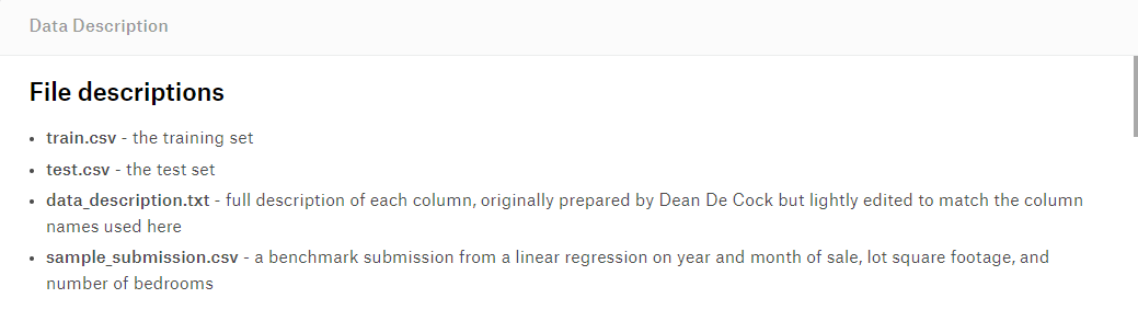
Kaggle平台上提供了训练集数据、测试集数据、数据描述文件、提交结果的样例文件,其中训练集数据是需要我们通过模型训练得出我们想来的模型来拟合数据,将测试集的内容输入到模型中得出结果。
4.初识数据
导入需要的相关包:
import numpy as np
import pandas as pd
import matplotlib.pyplot as plt
import seaborn as sns
from scipy import stats
from scipy.stats import norm, skew
%matplotlib inline
import warnings
warnings.filterwarnings('ignore')
导入数据,简单的观看下数据:
train = pd.read_csv('train.csv')
test = pd.read_csv('test.csv')
train.head()
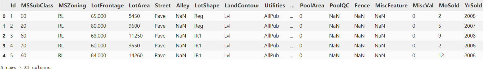
这里有81列,除去Id标识,以及SalePrice房产价格,正好79列。
再来看看数据各特征的确实情况:
train.info()
<class 'pandas.core.frame.DataFrame'>
RangeIndex: 1460 entries, 0 to 1459
Data columns (total 81 columns):
Id               1460 non-null int64
MSSubClass       1460 non-null int64
MSZoning         1460 non-null object
LotFrontage      1201 non-null float64
LotArea          1460 non-null int64
Street           1460 non-null object
Alley            91 non-null object
LotShape         1460 non-null object
LandContour      1460 non-null object
Utilities        1460 non-null object
LotConfig        1460 non-null object
LandSlope        1460 non-null object
Neighborhood     1460 non-null object
Condition1       1460 non-null object
Condition2       1460 non-null object
BldgType         1460 non-null object
HouseStyle       1460 non-null object
OverallQual      1460 non-null int64
OverallCond      1460 non-null int64
YearBuilt        1460 non-null int64
YearRemodAdd     1460 non-null int64
RoofStyle        1460 non-null object
RoofMatl         1460 non-null object
Exterior1st      1460 non-null object
Exterior2nd      1460 non-null object
MasVnrType       1452 non-null object
MasVnrArea       1452 non-null float64
ExterQual        1460 non-null object
ExterCond        1460 non-null object
Foundation       1460 non-null object
BsmtQual         1423 non-null object
BsmtCond         1423 non-null object
BsmtExposure     1422 non-null object
BsmtFinType1     1423 non-null object
BsmtFinSF1       1460 non-null int64
BsmtFinType2     1422 non-null object
BsmtFinSF2       1460 non-null int64
BsmtUnfSF        1460 non-null int64
TotalBsmtSF      1460 non-null int64
Heating          1460 non-null object
HeatingQC        1460 non-null object
CentralAir       1460 non-null object
Electrical       1459 non-null object
1stFlrSF         1460 non-null int64
2ndFlrSF         1460 non-null int64
LowQualFinSF     1460 non-null int64
GrLivArea        1460 non-null int64
BsmtFullBath     1460 non-null int64
BsmtHalfBath     1460 non-null int64
FullBath         1460 non-null int64
HalfBath         1460 non-null int64
BedroomAbvGr     1460 non-null int64
KitchenAbvGr     1460 non-null int64
KitchenQual      1460 non-null object
TotRmsAbvGrd     1460 non-null int64
Functional       1460 non-null object
Fireplaces       1460 non-null int64
FireplaceQu      770 non-null object
GarageType       1379 non-null object
GarageYrBlt      1379 non-null float64
GarageFinish     1379 non-null object
GarageCars       1460 non-null int64
GarageArea       1460 non-null int64
GarageQual       1379 non-null object
GarageCond       1379 non-null object
PavedDrive       1460 non-null object
WoodDeckSF       1460 non-null int64
OpenPorchSF      1460 non-null int64
EnclosedPorch    1460 non-null int64
3SsnPorch        1460 non-null int64
ScreenPorch      1460 non-null int64
PoolArea         1460 non-null int64
PoolQC           7 non-null object
Fence            281 non-null object
MiscFeature      54 non-null object
MiscVal          1460 non-null int64
MoSold           1460 non-null int64
YrSold           1460 non-null int64
SaleType         1460 non-null object
SaleCondition    1460 non-null object
SalePrice        1460 non-null float64
dtypes: float64(4), int64(34), object(43)
这里的数据的特征比较多,不宜观察确实的特征,选出确实特征。
lost = train.isnull().sum()
lost[lost > 0].sort_values(ascending=False)
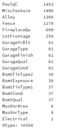
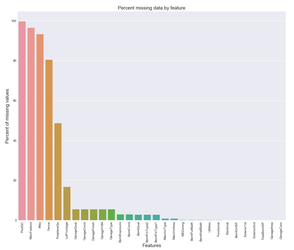
这里的缺失最多是PoolQC、MiscFeature、Alley、Fence,基本上大部分数据没有了,这种情况,一般会进行丢弃处理
5.可视化
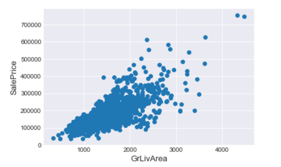
5.1.选取GrLivArea生活面积与房产价格进行可视化:
fig, ax = plt.subplots()
ax.scatter(x = train['GrLivArea'], y = train['SalePrice'])
plt.ylabel('SalePrice', fontsize=13)
plt.xlabel('GrLivArea', fontsize=13)
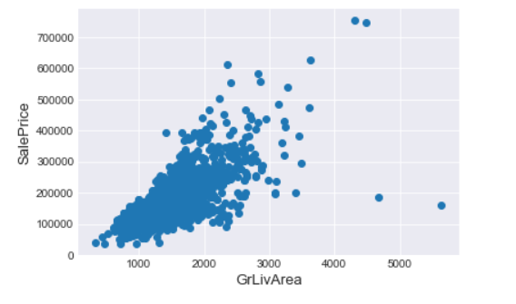
观察上面的散点图,发现有两个点,竟然出现较高的生活面积,却是较低的价格,如果这两个异常不加处理,将会影响模型的结果,当作丢弃出理。
train = train.drop(train[(train['GrLivArea']>4000)&(train['SalePrice']<300000)].index)

fig, ax = plt.subplots()
ax.scatter(train['GrLivArea'], train['SalePrice'])
plt.ylabel('SalePrice', fontsize=13)
plt.xlabel('GrLivArea', fontsize=13)
5.2.SalePrice房产是不是正态分布:
sns.distplot(train['SalePrice'], fit=norm);

(mu, sigma) = norm.fit(train['SalePrice'])
print('\n mu = {:.2f} and sigma = {:.2f}\n'.format(mu, sigma))

plt.legend(['Normal dist. ($\mu=$ {:.2f} and $\sigma=$ {:.2f})'.format(mu, sigma)], loc='best')
plt.ylabel('Frequency')
plt.title('SalePrice distribution')

fig = plt.figure()
res = stats.probplot(train['SalePrice'], plot=plt)
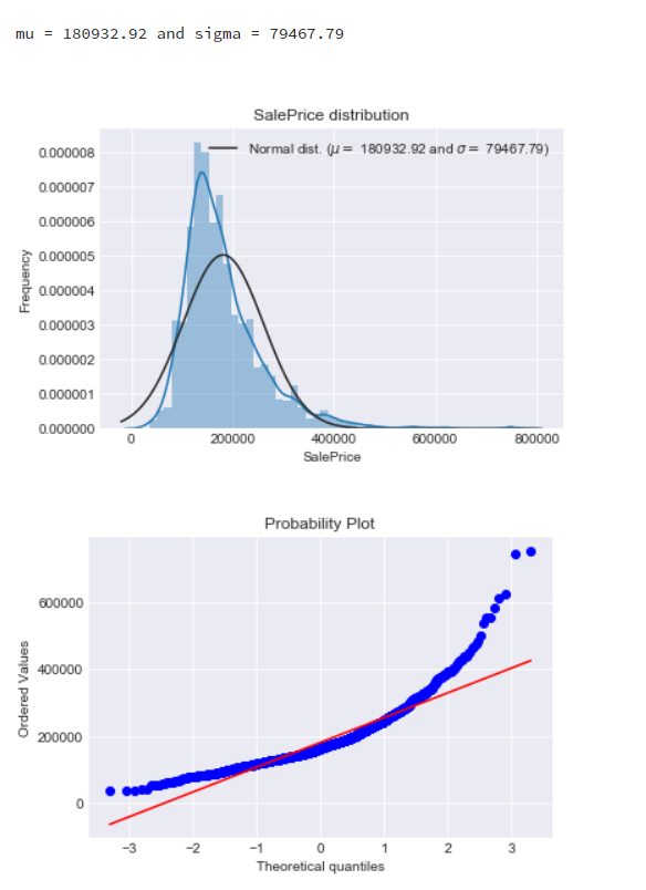
观察房产价格数据的条形图和Q-Q图,发现条形图出现了偏度,Q-Q图也不能拟合数据点,说明数据没有处于正态分布的情况,所以需要对数据进行转换。
由于SalePrice的数据比较大,所以将数据进行缩放处理,常用log函数:
train['SalePrice'] = np.log1p(train['SalePrice'])

sns.distplot(train['SalePrice'], fit=norm);

(mu, sigma) = norm.fit(train['SalePrice'])
print('\n mu = {:.2f} and sigma = {:.2f}\n'.format(mu, sigma))

plt.legend(['Normal dist. ($\mu=$ {:.2f} and $\sigma=$ {:.2f})'.format(mu, sigma)], loc='best')
plt.ylabel('Frequency')
plt.title('SalePrice distribution')

fig = plt.figure()
res = stats.probplot(train['SalePrice'], plot=plt)
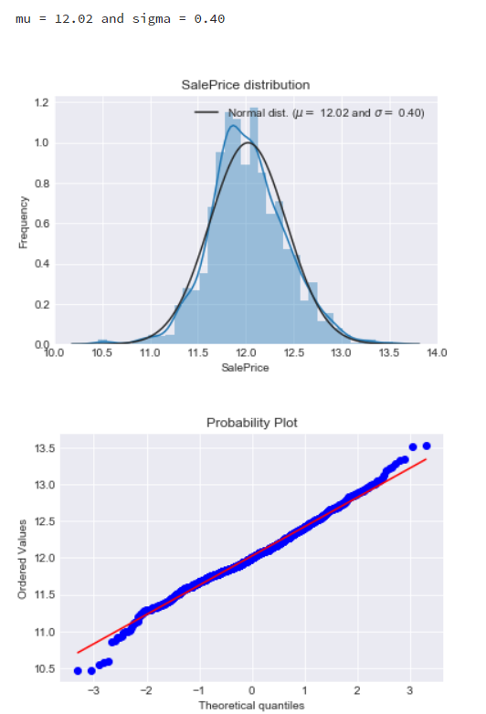
进行log变换后,发现数据满足了正态分布。
5.3.缺失情况的可视化:
all_data_na = (all_data.isnull().sum()/len(all_data)) * 100
all_data_na = all_data_na.drop(all_data_na[all_data_na == 0].index).sort_values(ascending=False)[:30]

f, ax = plt.subplots(figsize=(15, 12))
plt.xticks(rotation='90')
sns.barplot(x=all_data_na.index, y=all_data_na)
plt.xlabel('Features', fontsize=15)
plt.ylabel('Percent of missing values', fontsize=15)
plt.title('Percent missing data by feature', fontsize=15)
5.4.各项特征之间的相关性可视化:
corrmat = train.corr()
plt.subplots(figsize=(12, 9))
sns.heatmap(corrmat, vmax=0.9, square=True)
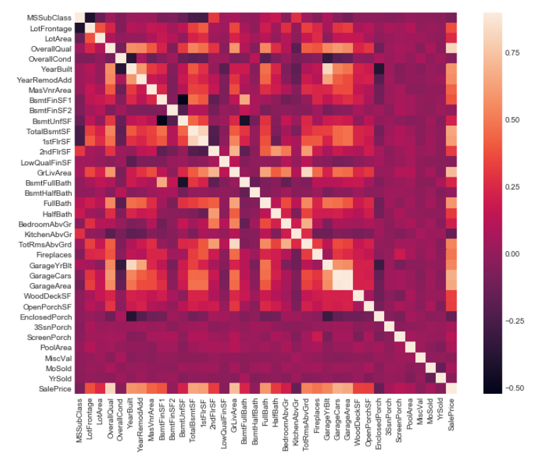
除了个别特征,相互之间的联系并不是特别明显。
6.特征工程
6.1.通过数据描述文件中,很多缺失的特征数据中NA意味着没有,查看数据类型,数据type分为object、int、float,如没有车库意味着没有车,以及相关的质量、类型都是没有的,用None、0来填充:
for col in ('GarageYrBlt', 'GarageArea', 'GarageCars', 'BsmtFinSF1', 'BsmtFinSF2', 'BsmtUnfSF', 'TotalBsmtSF', 'BsmtFullBath', 'BsmtHalfBath', 'MasVnrArea'):
    all_data[col] = all_data[col].fillna(0)
for col in ('GarageType', 'GarageFinish', 'GarageQual', 'GarageCond', 'PoolQC', 'MiscFeature', 'Alley', 'Fence', 'FireplaceQu', 'BsmtQual', 'BsmtCond', 'BsmtExposure', 'BsmtFinType1', 'BsmtFinType2', 'MasVnrType', 'MSSubClass'):
    all_data[col] = all_data[col].fillna('None')
还有没有说明是该房产没有该特征的数据,分为object、float类型,用众数、中位数来填充:
all_data['MSZoning'] = all_data['MSZoning'].fillna(all_data['MSZoning'].mode()[0])
all_data['Electrical'] = all_data['Electrical'].fillna(all_data['Electrical'].mode()[0])
all_data['KitchenQual'] = all_data['KitchenQual'].fillna(all_data['KitchenQual'].mode()[0])
all_data['Exterior1st'] = all_data['Exterior1st'].fillna(all_data['Exterior1st'].mode()[0])
all_data['Exterior2nd'] = all_data['Exterior2nd'].fillna(all_data['Exterior2nd'].mode()[0])
all_data['Functional'] = all_data['Functional'].fillna(all_data['Functional'].mode()[0])
6.2. Utilities:这个特征,由于大部分都是AllPub,而且在训练集中没有相关数据,所以可以删除:
all_data = all_data.drop(['Utilities'], axis=1)
6.3. 标准化标签,将str数据进行转化:
from sklearn.preprocessing import LabelEncoder
cols = ('FireplaceQu', 'BsmtQual', 'BsmtCond', 'GarageQual', 'GarageCond',
       'ExterQual', 'ExterCond', 'HeatingQC', 'PoolQC', 'KitchenQual', 'BsmtFinType1',
       'BsmtFinType2', 'Functional', 'Fence', 'BsmtExposure', 'GarageFinish', 'LandSlope',
       'LotShape', 'PavedDrive', 'Street', 'Alley', 'CentralAir', 'MSSubClass',
       'OverallCond', 'YrSold', 'MoSold')
for c in cols:
    lbl = LabelEncoder()
    lbl.fit(list(all_data[c].values))
    all_data[c] = lbl.transform(list(all_data[c].values))
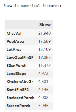
6.4. 非object类型数据的偏度情况:
numeric_feats = all_data.dtypes[all_data.dtypes != 'object'].index

skewed_feats = all_data[numeric_feats].apply(lambda x: skew(x.dropna())).sort_values(ascending=False)
print("\nSkew in numerical features: \n")
skewness = pd.DataFrame({'Skew': skewed_feats})
skewness.head(10)
将不满足正态分布的数据转换成正态分布情况:
skewness = skewness[abs(skewness) > 0.75]
transform".format(skewness.shape[0]))

from scipy.special import boxcox1p
skewed_features = skewness.index
lam = 0.15
for feat in skewed_features:
    all_data[feat] = boxcox1p(all_data[feat], lam)
7.建立模型:
导入相关模型包:
from sklearn.linear_model import ElasticNet, Lasso, BayesianRidge, LassoLarsIC
from sklearn.ensemble import RandomForestRegressor,GradientBoostingRegressor
from sklearn.kernel_ridge import KernelRidge
from sklearn.pipeline import make_pipeline
from sklearn.preprocessing import RobustScaler
from sklearn.base import BaseEstimator, TransformerMixin, RegressorMixin, clone
from sklearn.model_selection import KFold, cross_val_score, train_test_split
from sklearn.metrics import mean_squared_error
n_folds = 5
def rmsle_cv(model):
    kf = KFold(n_folds, shuffle=True, random_state=42).get_n_splits(train.values)
    rmse = np.sqrt(-cross_val_score(model, train.values, y_train, scoring='neg_mean_squared_error', cv=kf))
    return rmse

lasso = make_pipeline(RobustScaler(), Lasso(alpha=0.0005, random_state=1))

ENet = make_pipeline(RobustScaler(), ElasticNet(alpha=0.0005, l1_ratio=.9, random_state=3))

KRR = KernelRidge(alpha=0.6, kernel='polynomial', degree=2, coef0=2.5)

GBoost = GradientBoostingRegressor(n_estimators=3000, learning_rate=0.05,
                                  max_depth=4, max_features='sqrt',
                                  min_samples_leaf=15, min_samples_split=10,
                                  loss='huber', random_state=5)

score = rmsle_cv(lasso)
print("Lasso score: {:.4f} ({:.4f})".format(score.mean(), score.std()))

score = rmsle_cv(ENet)
print("ElasticNet score: {:.4f} ({:.4f})".format(score.mean(), score.std()))

score = rmsle_cv(KRR)
print("Kernel Ridge score: {:.4f} ({:.4f})".format(score.mean(), score.std()))

score = rmsle_cv(GBoost)
print("Gradient Boosting score: {:.4f} ({:.4f})".format(score.mean(), score.std()))
Lasso score: 0.1115 (0.0074)

ElasticNet score: 0.1116 (0.0074)

Kernel Ridge score: 0.1153 (0.0075)

Gradient Boosting score: 0.1177 (0.0080)
综合模型的平均得分:
class AveragingModels(BaseEstimator, RegressorMixin, TransformerMixin):
    def __init__(self, models):
        self.models = models

    def fit(self, X, y):
        self.models_ = [clone(x) for x in self.models]

        for model in self.models_:
            model.fit(X, y)
        return self

    def predict(self, X):
        predictions = np.column_stack([
            model.predict(X) for model in self.models_
        ])
        return np.mean(predictions, axis=1)

averaged_models = AveragingModels(models=(ENet, GBoost, KRR, lasso))

score = rmsle_cv(averaged_models)
print("Averaged base models score: {:.4f}({:.4f})\n".format(score.mean(), score.std()))
Averaged base models score: 0.1091(0.0075)

综上得到模型的平均误差为:0.1091

 浙公网安备 33010602011771号