GAN 对抗神经网络(Generative Adversarial Networks)

GAN 对抗神经网络 小案例

GAN存在目的:

     为了通过一定的手段，模拟出一种数据的概率分布的生成器(生成手段)，使得这种概率分布与 某种观测数据的概率统计分布一致或者尽可能接近。

GAN的厉害之处在于，它的学习性质是无监督的。GAN不需要标记数据，这使GAN功能强大，因为数据标记的工作极其枯燥繁琐。

原理

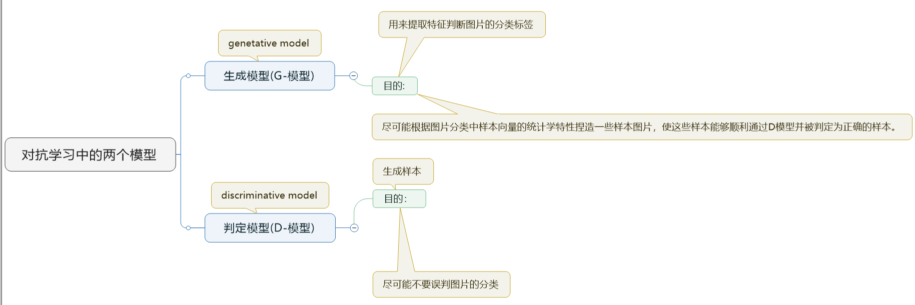
GAN是一种生成式对抗网络，它属于一种生成式网络，它的对抗性主要由两个网络体现，一个D网络和一个G网络

D网络称为判别器，它的职责是尽量区分开真实样本和生成样本。

G网络称为生成器，它的职责是尽量生成接近真实的样本，让判别器判别G网络生成的样本是真实的。

训练模型

        '''
1.导入必要的库

'''

import os

os.environ['TF_CPP_MIN_LOG_LEVEL'] = '2'
os.environ["CUDA_DEVICE_ORDER"] = "PCI_BUS_ID"
os.environ["CUDA_VISIBLE_DEVICES"] = "1"  # 指定第一块gpu

# 参数解析包
import argparse
#
import numpy as np
from scipy.stats import norm  # scipy 数值计算库
# tensorflow 包
import tensorflow as tf
# 可视化包
import matplotlib.pyplot as plt
from matplotlib import animation
import seaborn as sns  # 数据模块可视化

sns.set(color_codes=True)  # 设置主题颜色

# 设置种子，用于随机初始化
seed = 42

# 设置随机数，使得每次生成的随机数相同
np.random.seed(seed)
tf.set_random_seed(seed)
'''
2.定义样本分布以及生成样本分布

样本分布使用均值为4，方差为0.5的高斯分布

生成样本分布采用均匀加噪处理

'''


# 定义真实的数据分布，这里为高斯分布
class DataDistribution(object):
    def __init__(self):
        # 高斯分布参数
        # 均值为4
        # 标准差为0.5
        self.mu = 4  # 均值
        self.sigma = 0.5  # 标准差

    def sample(self, N):
        samples = np.random.normal(self.mu, self.sigma, N)
        samples.sort()
        return samples


# 随机初始化一个分布，做为G网络的输入
class GeneratorDistribution(object):  # 在生成模型额噪音点，初始化输入
    def __init__(self, range):
        self.range = range

    def sample(self, N):
        return np.linspace(-self.range, self.range, N) + \
               np.random.random(N) * 0.01


'''
3.定义网络线性运算y=wx+b

代码实现了输入样本x，执行y=wx+b的运算，其中norm和const是初始化w和b的分布，使用tf.variable_scope()定义名字空间，有利于简化代码
'''


# 定义线性运算函数，其中参数output_dim=h_dim*2=8
def linear(input, output_dim, scope=None, stddev=1.0):
    # 定义一个随机初始化
    norm = tf.random_normal_initializer(stddev=stddev)
    # b初始化为0
    const = tf.constant_initializer(0.0)
    with tf.variable_scope(scope or 'linear'):
        # 声明w的shape,输入为（12，1）*w，故w为（1，8），w的初始化方式为高斯初始化
        w = tf.get_variable('w', [input.get_shape()[1], output_dim], initializer=norm)
        # b初始化为常量
        b = tf.get_variable('b', [output_dim], initializer=const)
        # 执行线性运算
        return tf.matmul(input, w) + b


'''
4.定义生成网络和判别网络
生成网络:
生成网络是两层的感知器，第一层使用softplus函数来处理输入，
第二层即使用简单的线性运算生成数据

判别网络：

判别网络使用具有4层的深度网络，
由于判别网络许需要具有足够的判别能力才能促使生成网络生成更好的样本，
所以判别网络在每一层都是用tanh()函数作为激活，最后一层使用sigmoid函数输出。


'''


# 生成器

def generator(input, h_dim):
    h0 = tf.nn.softplus(linear(input, h_dim, 'g0'))
    h1 = linear(h0, 1, 'g1')
    return h1  # z最后的生成模型


# 判别器
# 初始化w和b的函数，其中h0,h1,h2,h3为层，将mlp_hidden_size=4传给h_dim
def discriminator(input, h_dim):
    # linear 控制初始化参数
    # linear 控制w和b的初始化,这里linear函数的第二个参数为4*2=8
    # 第一层
    h0 = tf.tanh(linear(input, h_dim * 2, 'd0'))
    # 第二层输出，隐藏层神经元个数还是为8
    h1 = tf.tanh(linear(h0, h_dim * 2, 'd1'))
    # h2为第三层输出值
    h2 = tf.tanh(linear(h1, h_dim * 2, scope='d2'))
    # 最终的输出值 对判别网络输出
    h3 = tf.sigmoid(linear(h2, 1, scope='d3'))
    return h3


'''
5.定义优化器
生成模型、判别模型和预训练生成器模型都使用同一个优化器，
该优化器使用学习速度下降的方法，
并使用通常的梯度下降学习器。
'''


# 优化器  采用学习率衰减的方法
def optimizer(loss, var_list, initial_learning_rate):
    decay = 0.95
    num_decay_steps = 150
    batch = tf.Variable(0)
    # 调用学习率衰减的函数
    learning_rate = tf.train.exponential_decay(
        initial_learning_rate,
        batch,
        num_decay_steps,
        decay,
        staircase=True
    )
    # 梯度下降求解
    optimizer = tf.train.GradientDescentOptimizer(learning_rate).minimize(
        loss,
        global_step=batch,
        var_list=var_list
    )
    return optimizer


class GAN(object):
    def __init__(self, data, gen, num_steps, batch_size, log_every):
        self.data = data
        self.gen = gen
        self.num_steps = num_steps
        self.batch_size = batch_size
        self.log_every = log_every
        # 隐层神经元个数
        self.mlp_hidden_size = 4
        # 学习率
        self.learning_rate = 0.03
        # 通过placeholder格式来创造模型
        self._create_model()

    '''
        6.创建模型
        模型都定义好了，优化器选择完毕，则创建训练模型。
        里包括三个模型D_pre、Gen和Dist，分别为判别器预训练模型，生成模型和判别模型，由于判别器需要有较好的性能才能进行生成对抗，所以提前对判别器进行预训练，可以达到很好的效果。
        创建计算图，对三种网络模型定义网络参数，包括输入、输出、损失函数、优化器等。       
        
    '''

    def _create_model(self):
        # 创建一个名叫D_pre的域，先构造一个D_pre网络，用来训练出真正D网络初始化网络所需要的参数
        with tf.variable_scope('D_pre'):  # 构造D_pre模型骨架,预先训练,为了去初始化真正的判别模型
            # 输入的shape为（12，1），一个batch一个batch的训练，每个batch的大小为12，要训练的数据为1维的点
            self.pre_input = tf.placeholder(tf.float32, shape=(self.batch_size, 1))

            self.pre_labels = tf.placeholder(tf.float32, shape=(self.batch_size, 1))
            # 调用discriminator来初始化w和b参数,其中self.mlp_hidden_size=4，为discriminator函数的第二个参数
            D_pre = discriminator(self.pre_input, self.mlp_hidden_size)
            # 预测值和label之间的差异
            self.pre_loss = tf.reduce_mean(tf.square(D_pre - self.pre_labels))
            # 定义优化器求解
            self.pre_opt = optimizer(self.pre_loss, None, self.learning_rate)

        # This defines the generator network - it takes samples from a noise
        # distribution as input, and passes them through an MLP.
        # 真正的G网络
        with tf.variable_scope('Gen'):  # 生成模型
            self.z = tf.placeholder(tf.float32, shape=(self.batch_size, 1))  # 噪音的输入
            # 生成网络只有两层
            self.G = generator(self.z, self.mlp_hidden_size)  # 最后的生成结果

        # The discriminator tries to tell the difference between samples from the
        # true data distribution (self.x) and the generated samples (self.z).
        #
        # Here we create two copies of the discriminator network (that share parameters),
        # as you cannot use the same network with different inputs in TensorFlow.
        # D网络
        with tf.variable_scope('Disc') as scope:  # 判别模型 不光接受真实的数据 还要接受生成模型的判别
            self.x = tf.placeholder(tf.float32, shape=(self.batch_size, 1))
            # 构造D1网络，真实的数据
            self.D1 = discriminator(self.x, self.mlp_hidden_size)  # 真实的数据
            # 重新使用一下变量，不用重新定义
            scope.reuse_variables()  # 变量重用
            # D2，生成的数据
            self.D2 = discriminator(self.G, self.mlp_hidden_size)  # 生成的数据

        # Define the loss for discriminator and generator networks (see the original
        # paper for details), and create optimizers for both
        # 定义判别网络的损失函数
        self.loss_d = tf.reduce_mean(-tf.log(self.D1) - tf.log(1 - self.D2))
        # 生定义成网络的损失函数,希望其趋向于1
        self.loss_g = tf.reduce_mean(-tf.log(self.D2))

        self.d_pre_params = tf.get_collection(tf.GraphKeys.TRAINABLE_VARIABLES, scope='D_pre')
        self.d_params = tf.get_collection(tf.GraphKeys.TRAINABLE_VARIABLES, scope='Disc')
        self.g_params = tf.get_collection(tf.GraphKeys.TRAINABLE_VARIABLES, scope='Gen')
        # 优化，得到两组参数
        self.opt_d = optimizer(self.loss_d, self.d_params, self.learning_rate)
        self.opt_g = optimizer(self.loss_g, self.g_params, self.learning_rate)

    '''
        7.执行训练
        
        首先初始化参数，其次抽取样本执行判别器预训练，
        将与训练的模型参数拷贝到判别模型，
        然后对抗训练判别模型和生成模型
    
    '''

    def train(self):
        with tf.Session() as session:
            tf.global_variables_initializer().run()

            # pretraining discriminator
            # 先训练D_pre网络
            num_pretrain_steps = 1000  # 迭代次数，先训练D_pre ,先让其有一个比较好的初始化参数
            for step in range(num_pretrain_steps):
                # 随机生成数据
                d = (np.random.random(self.batch_size) - 0.5) * 10.0
                labels = norm.pdf(d, loc=self.data.mu, scale=self.data.sigma)
                pretrain_loss, _ = session.run([self.pre_loss, self.pre_opt], {  # 相当于一次迭代
                    self.pre_input: np.reshape(d, (self.batch_size, 1)),
                    self.pre_labels: np.reshape(labels, (self.batch_size, 1))
                })
                # 拿出预训练好的数据
            self.weightsD = session.run(self.d_pre_params)  # 相当于拿到之前的参数
            # copy weights from pre-training over to new D network
            for i, v in enumerate(self.d_params):
                session.run(v.assign(self.weightsD[i]))  # 把权重参数拷贝
            # 训练真正的生成对抗网络
            for step in range(self.num_steps):
                # update discriminator
                x = self.data.sample(self.batch_size)  # 真实的数据
                # z是一个随机生成的噪音
                z = self.gen.sample(self.batch_size)  # 随意的数据，噪音点
                # 优化判别网络
                loss_d, _ = session.run([self.loss_d, self.opt_d], {  # D两种输入真实，和生成的
                    self.x: np.reshape(x, (self.batch_size, 1)),
                    self.z: np.reshape(z, (self.batch_size, 1))
                })

                # update generator 更新生成器
                z = self.gen.sample(self.batch_size)  # G网络
                # 迭代优化
                loss_g, _ = session.run([self.loss_g, self.opt_g], {
                    self.z: np.reshape(z, (self.batch_size, 1))
                })

                # 打印
                if step % self.log_every == 0:
                    print('{}: {}\t{}'.format(step, loss_d, loss_g))
                    # 画图
                if step % 100 == 0 or step == 0 or step == self.num_steps - 1:
                    self._plot_distributions(session)

    def _samples(self, session, num_points=10000, num_bins=100):
        xs = np.linspace(-self.gen.range, self.gen.range, num_points)
        bins = np.linspace(-self.gen.range, self.gen.range, num_bins)

        # data distribution
        d = self.data.sample(num_points)
        pd, _ = np.histogram(d, bins=bins, density=True)

        # generated samples
        zs = np.linspace(-self.gen.range, self.gen.range, num_points)
        g = np.zeros((num_points, 1))
        for i in range(num_points // self.batch_size):  # 整数除法   这是python 语法规定的
            g[self.batch_size * i:self.batch_size * (i + 1)] = session.run(self.G, {
                self.z: np.reshape(
                    zs[self.batch_size * i:self.batch_size * (i + 1)],
                    (self.batch_size, 1)
                )
            })
        pg, _ = np.histogram(g, bins=bins, density=True)

        return pd, pg

    def _plot_distributions(self, session):
        pd, pg = self._samples(session)
        p_x = np.linspace(-self.gen.range, self.gen.range, len(pd))
        f, ax = plt.subplots(1)
        ax.set_ylim(0, 1)
        plt.plot(p_x, pd, label='real data')
        plt.plot(p_x, pg, label='generated data')
        plt.title('1D Generative Adversarial Network')
        plt.xlabel('Data values')
        plt.ylabel('Probability density')
        plt.legend()
        plt.show()


def main(args):
    model = GAN(
        # 定义真实数据的分布
        DataDistribution(),
        # 创造一些噪音点，用来传入G函数
        GeneratorDistribution(range=8),
        # 迭代次数
        args.num_steps,
        # 一次迭代12个点的数据
        args.batch_size,
        # 隔多少次打印当前loss
        args.log_every,
    )
    model.train()


def parse_args():
    parser = argparse.ArgumentParser()
    parser.add_argument('--num-steps', type=int, default=1200,
                        help='the number of training steps to take')
    parser.add_argument('--batch-size', type=int, default=12,
                        help='the batch size')
    parser.add_argument('--log-every', type=int, default=10,
                        help='print loss after this many steps')
    return parser.parse_args()


if __name__ == '__main__':
    main(parse_args())

'''
参考文献
    https://www.cnblogs.com/LHWorldBlog/p/9250419.html

'''