神经网络笔记

Tensorflow 官方文档

http://www.tensorfly.cn/tfdoc/api_docs/python/nn.html

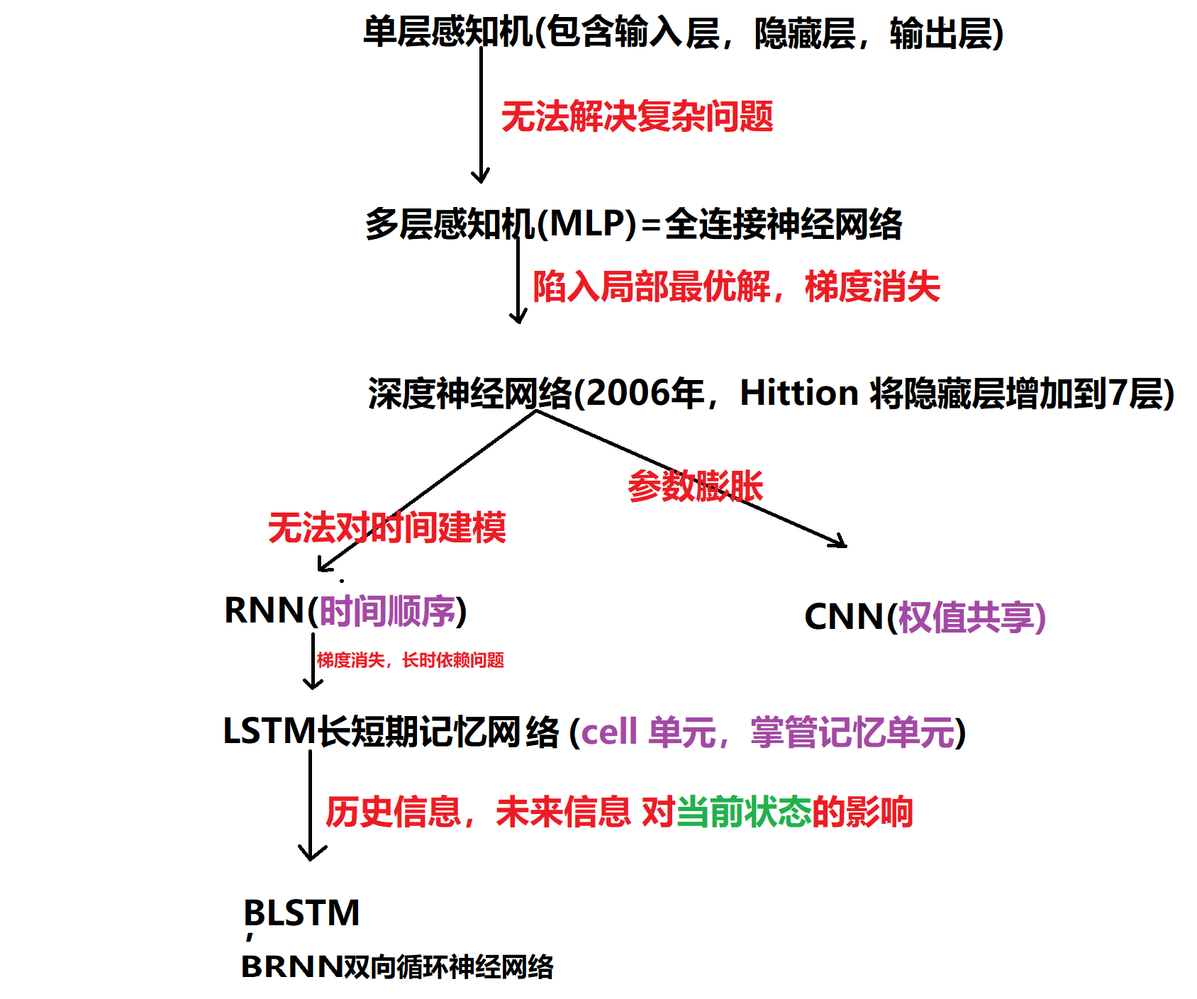
神经网络分类

参考文献

https://blog.csdn.net/lff1208/article/details/77717149

https://www.leiphone.com/news/201702/ZwcjmiJ45aW27ULB.html

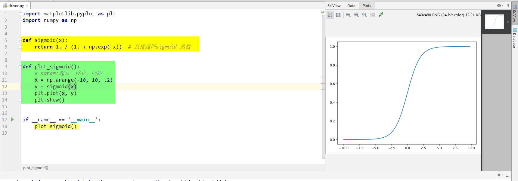
Python3用matplotlib绘制sigmoid函数

双曲余弦 双曲正弦 双曲正切

import numpy as np
import matplotlib.pyplot as plt

plt.rcParams['font.sans-serif'] = ['SimHei']  # 用来正常显示中文标签
plt.rcParams['axes.unicode_minus'] = False  # 用来正常显示负号


def plot_tanh():
    # linspace的第一个参数表示起始点，第二个参数表示终止点，第三个参数表示数列的个数
    # x = np.linspace(-10, 10, 1000)
    # x = np.arange(-10, 10, .002)
    x = np.arange(-10, 10, .002)
    y = np.tanh(x)
    plt.plot(x, y,label='label2',color="red",linewidth=2)

    plt.xlabel("abscissa横坐标")
    plt.ylabel("ordinate纵坐标")
    plt.title("双曲图")
    plt.show()
def plot_sinh():
    # linspace的第一个参数表示起始点，第二个参数表示终止点，第三个参数表示数列的个数
    # x = np.linspace(-10, 10, 1000)
    # x = np.arange(-10, 10, .002)
    x = np.arange(-10, 10, .002)
    y = np.sinh(x)
    plt.plot(x, y,label='label',color="green",linewidth=6)

    plt.xlabel("abscissa横坐标")
    plt.ylabel("ordinate纵坐标")
    plt.title("双曲图")
    plt.show()

def plot_cosh():
    # linspace的第一个参数表示起始点，第二个参数表示终止点，第三个参数表示数列的个数
    x = np.linspace(-10, 10, 1000)
    # x = np.arange(-10, 10, .002)
    # x = np.arange(-10, 10, .002)
    y = np.cosh(x)
    plt.plot(x, y,label='label3',color="blue",linewidth=9)

    plt.xlabel("abscissa横坐标")
    plt.ylabel("ordinate纵坐标")
    plt.title("双曲图")
    plt.show()
def plot_coth():
    # linspace的第一个参数表示起始点，第二个参数表示终止点，第三个参数表示数列的个数
    x = np.linspace(-10, 10, 1000)
    # x = np.arange(-10, 10, .002)
    # x = np.arange(-10, 10, .002)
    y = (np.cosh(x)/np.sinh(x))
    plt.plot(x, y,label='label4',color="yellow",linewidth=9)

    plt.xlabel("abscissa横坐标")
    plt.ylabel("ordinate纵坐标")
    plt.title("双曲图")
    plt.show()


if __name__ == '__main__':
    # plot_tanh()
    # plot_sinh()
    # plot_cosh()
    plot_coth()

利用tensorflow 接口实现常见的激活函数图

import matplotlib.pyplot as plt
import numpy as np
import tensorflow as tf

#  Your CPU supports instructions that this TensorFlow binary was not compiled to use: AVX2
import os

os.environ['TF_CPP_MIN_LOG_LEVEL'] = '2'
# 解决乱码手段
plt.rcParams['font.sans-serif'] = ['SimHei']  # 用来正常显示中文标签
plt.rcParams['axes.unicode_minus'] = False  # 用来正常显示负号


def plot_sigmoid():
    x = tf.constant(np.arange(-10, 10, .2), dtype=tf.float32)
    print(x)
    sess = tf.Session()
    print(sess)
    # y=sess.run(tf.log_sigmoid(x))
    y = sess.run(tf.sigmoid(x))  # sigmoid激活函数
    y1 = sess.run(tf.tanh(x))  # tanh激活函数
    # y2 = sess.run(tf.nn.relu(x))  # relu激活函数

    print(y)
    print(y1)
    # print(y2)
    plt.plot(np.arange(-10, 10, .2), y)
    plt.plot(np.arange(-10, 10, .2), y1)
    # plt.plot(np.arange(-10, 10, .2), y2)

    plt.xlabel("abscissa横坐标")
    plt.ylabel("ordinate纵坐标")
    plt.title("常见各种激活函数")

    plt.show()


if __name__ == '__main__':
    plot_sigmoid()

Softmax激励函数

import matplotlib.pyplot as plt
import numpy as np
import tensorflow as tf

#  Your CPU supports instructions that this TensorFlow binary was not compiled to use: AVX2
# s.environ["TF_CPP_MIN_LOG_LEVEL"]='1' # 这是默认的显示等级，显示所有信息  
# os.environ["TF_CPP_MIN_LOG_LEVEL"]='2' # 只显示 warning 和 Error   
# os.environ["TF_CPP_MIN_LOG_LEVEL"]='3' # 只显示 Error


import os

os.environ['TF_CPP_MIN_LOG_LEVEL'] = '1'
# 解决乱码手段
plt.rcParams['font.sans-serif'] = ['SimHei']  # 用来正常显示中文标签
plt.rcParams['axes.unicode_minus'] = False  # 用来正常显示负号


def plot_Softmax():
    x = tf.constant(np.arange(-10, 10, .2), dtype=tf.float32)
    print(x)
    sess = tf.Session()
    print(sess)
    y = sess.run(tf.nn.softmax(x))  # Softmax激活函数

    print(y)

    plt.plot(np.arange(-10, 10, .2), y)

    plt.xlabel("abscissa横坐标")
    plt.ylabel("ordinate纵坐标")
    plt.title("Softmax  激活函数")

    plt.show()


if __name__ == '__main__':
    plot_Softmax()

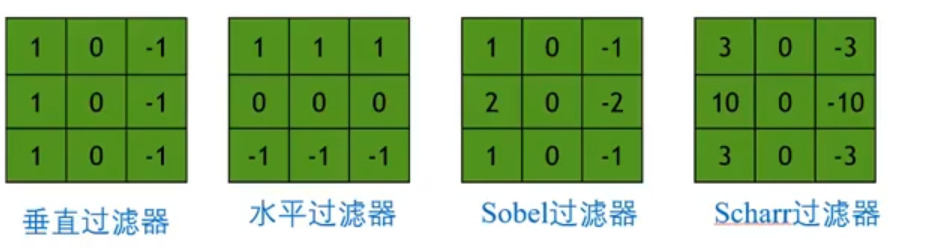
水平卷积核/垂直卷积核(过滤器和卷积核是一个意思)

padding

通过一个3*3的卷积核来对6*6的图像进行卷积，得到了一幅4*4的图像。
假设输入/原始图像大小为n*n，过滤器大小为f*f，则输出图像大小则为（n-f+1）*（n-f+1）。
这样做卷积运算的缺点：（1）卷积图像的大小会不断缩小；（2）丢掉了很多图像边缘的信息。

卷积神经网络CNN参考文献

https://blog.csdn.net/ice_actor/article/details/78648780