社会科学问题研究的计算实践——6、网络效应(计算实践:网络效应下的价格策略比较)
 计算实践:网络效应下的价格策略比较
学习资源来自,一个哲学学生的计算机作业 (karenlyu21.github.io)
1、背景问题
经济学中最经典的讨论中,市场没有网络效应。也就是说,每个人评估一个物品的价值不受他人影响。每个人只需要根据价格和自己的估值决定是否购买。但无网络效应的假设不是普遍适用的。对于某些产品,例如传真机、微信,如果使用的人不多,一个人会觉得这个产品没什么价值;随着参与人增多,其他人也纷纷被其价值吸引而参与。这就是“网络效应”。对于有网络效应的产品,产品推广、扩大用户规模具有特殊意义
1.1、均衡求解
为了进一步分析有网络效应的市场,我们定义如下三个变量:
- 价格p。
- 用户x,定义在[0,1]:一个买家在市场中的位置,其数值表示对产品的估值比x高的人占总人数的比例。x=0对应的是对产品估值最高的人,x=1对应的是对产品估值最低的人。
- 预期规模z,定义在[0,1]:人们对于产品使用人数规模的预期。我们假定所有人的预期相等(这是市场的公共知识)。z=0时,大家预期没有人会使用该产品;z=1时,大家预期所有人都会使用。
为了分析用户的购买行为,我们定义如下两个函数:
- 保留价函数r(x):无网络效应时,产品对用户x的价值;
- 规模放大因子f(z):当预期总人数(规模)为z时,网络效应导致产品对用户x的价值增加,f(z)表示增幅大小。
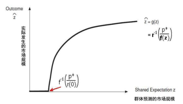
那么,r(x)f(z)表示在预期规模z下产品对用户x的价值。当且仅当r(x)f(z)≥p时,x会购买该产品。
在这个市场里,均衡在何处达成?
为了简化分析,设
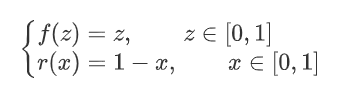
考虑z=0.6的情境,供需情况如下。
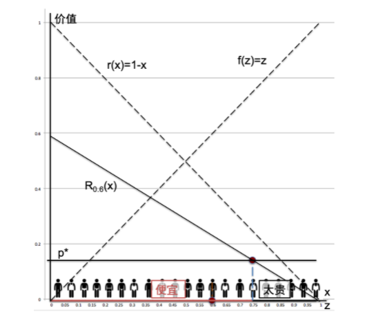
当z=0.6时,实际上愿意购买产品的人达到了0.75(均衡点左侧的人觉得该商品比较便宜、愿意买;右边的人不愿意买)。人们会根据实际情况调整预期,这导致f(z)的值会发生变化,z=0.6无法达成均衡。
假设人们用上一轮的实际规模更新自己的预期,新一轮的预期规模则为0.75。重新计算供需情况,我们会发现,z=0.75同样无法达成均衡。
当预期规模z与实际规模z^相等

时,市场的供需情况不会再发生变化,此时达成均衡。设x0是愿意购买的人中保留价最低的,即

x0的保留价最低意味着x0刚刚好愿意购买,亦即他对产品的估值恰好等于产品的定价

联立(1)(2)(3),得到

这一方程的解就是市场均衡。如下图所示,它一般存在两个解,不稳定均衡点z^′ 和 稳定均衡点z^″。
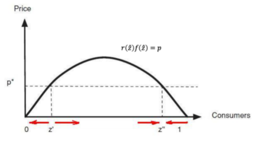
在这一分析过程中,我们看到,预期规模超过z′后,实际规模会随之更高,直到二者相等(对应到上图,就是由从左到右逼近z″的红色箭头),达到所谓预期的自我实现(self-fulfilling)。
1.2、市场动力学:达成均衡的动态过程
现在我们更详细地考虑达成均衡的过程,在此过程中,人们根据市场情况调整预期,实际规模又随之变化,循环往复。
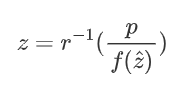
达成均衡的过程中,市场处在不均衡状态。在等式(1)(2)(3)中,条件x0=z^ 在非均衡情况中不成立。此时我们只需要联立(1)(3),得到预期规模z和实际规模z^的关系
此外,z≥0。那么,z与z^ 的关系可以用下图表示:
根据均衡求解的假设,同时不妨假设人们以月为单位来观察市场并做出预测,人们对于下月市场规模的预期等于上月的实际规模

那么,市场规模的动态变化就如下图所示。
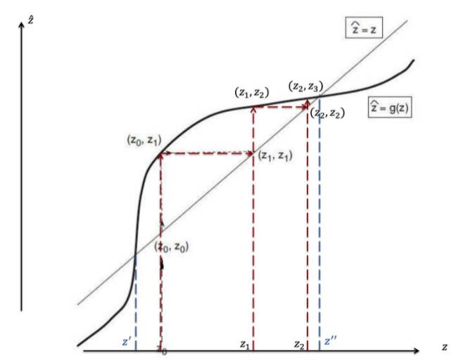
(由于人们根据上月实际规模调整预期,我们得到上月实际规模以后平行于x轴作线,遇到z^=z 后折返,交点所对应的横坐标等于上月实际规模,亦即下月预期规模,与z^ =g(z)的交点即为下月实际规模。)
上图的例子中,市场的动态发展趋向z^=z 与 z^=g(z)的交点z″ ,这也是上文提到的稳定平衡点。由于z′ 是不稳定平衡点,如果初始预期规模z0 >z′ ,最终的均衡点都在z″ ;而如果z0<z′ ,市场规模会不断减小至0。——这意味着,在有网络效应的市场中,初始规模非常重要。
那么,什么样的定价行为能最大化卖家利润呢?我们发现,当定价足够低,不稳定均衡点可能不复存在。
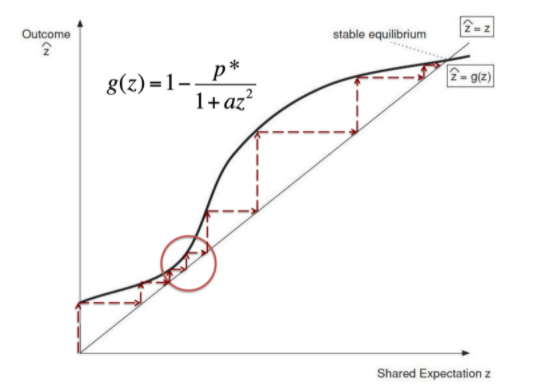
这种情况下,消费者的行为将推动市场自动成长,直到高端稳定均衡点。这种定价策略打开了一个市场自动成长的通道!
2、 计算实践:网络效应下的价格策略比较
2.1、作业描述与算法思路
在背景问题中,我们看到,对于有网络效应的产品,不同定价策略会影响市场的动态变化、影响商家的利润。本次作业,我们就是要模拟不同定价策略的效果。
考虑你开发了一个具有网络效应的信息服务产品,有如下特点
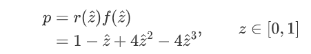
- 市场保留价函数r(x)=1−x,网络效应函数为f(z)=1+4z2,都定义在区间[0,1]。
- 该服务拟按照以月为单位订阅的方式收费,意味着每个月你可能调整一次价格。假设潜在的用户都是在月初同步做决定,都能看到上个月的市场规模。
- 市场最初对用户规模的预期为0。
- 假设你每月服务一个用户的成本是0.2。
试模拟这个市场运行n个月(n=10,20,30,…,100),观察在不同的价格p策略下,你可能得到的利润情况:
- 固定价格策略:固定p=0.5。
- 规模价格策略:假设初始价格是0.5,然后让p随市场规模的改变线性调整:(本月规模−上月规模)>0,下月的p提高20;(本月规模−上月规模)<0,则降低20;(本月规模−上月规模)=0,则保持。
- 贪心策略:每个月都采用一个能带来当月最大利润的价格。
- 试试能否考虑一个不同的策略,得到更好的结果。
我的算法思路如下:
- 首先需要定义价格函数,能根据各策略的要求返回当月价格。
- 根据当月的价格和上月规模(当月的预期规模),我们能够计算出当月的实际规模和利润,进而计算多月内的总利润。
在老师提示的三种策略中,贪心策略的算法相对复杂。
首先,我们根据市场保留价函数r(x)=1−x,网络效应函数为f(z)=1+4z2,可以求得实际规模z^与预期规模z的关系为

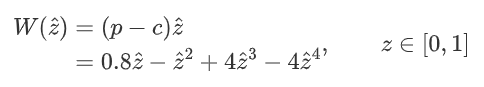
我们要最大化当月利润(设为第i月),它可以用(每个人所付价钱−服务每个人的成本)×市场规模
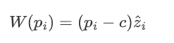
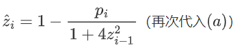
来表示,再代入(a),可以得到
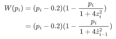
这一函数求导,我们可以得到当
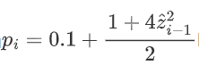
时,W(pi)取到最大值。贪心策略就根据这一公式返回每月的定价。
一个策略是固定高价策略,即每个月的定价固定在0.9。
另一个策略是耐心策略,作为对贪心策略的改良。贪心策略目光短浅,仅仅致力于最大化当月利润,却可能因此减小市场规模,导致长期利润大幅减少。为了避免追求最大利润时提价太多,我在确定当月价格时,计算该价格pi保持两个月后次月的利润Wi+1,并使其最大化。
首先,次月(第i+1月)的利润可以表示为
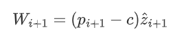
由于i月的价格pi一直保持到i+1月,pi+1=pi。再代入(a),有
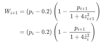
其中,
把Wi+1表示为关于pi的函数后,我们就可以利用scipy库,求出Wi+1最大时的pi ∗。
贪心策略的过幅提价在这一策略中不会发生,因为过幅提价会导致次月利润大幅减小。
此外,我还把初始阶段的价格设为0.9,等市场增长到稳定均衡点后,我再确定次月利润最大时的定价。
2.2、编程实现与要点说明
2.2.1、定价函数
定义固定价格策略的定价函数。无论输入为何,该函数总是返回0.5的固定价格。
def stable(p0, z1, z2, rnd):  # monthly prize stablized at 0.5
    return 0.5
定义规模价格策略的定价函数。输入上月价格p0、上月规模z2、上上月规模z1,按照题目要求、根据两个月之间规模的变化调整价格。
def scaled(p0, z1, z2, rnd):  # if the scale increases, the price increases accordingly
    # p0: the price of last month
    # z1: the scale of the month before the last month
    # z2: the scale of the last month
    if z1 == None:
        return 0.5
    elif z1 < z2:
        return 1.2 * p0
    elif z1 > z2:
        return 0.8 * p0
    else:
        return p0
定义贪心策略的定价函数。
输入上月实际规模z2,返回一个能够最大化当月利润的价格。根据上文的分析,这一价格应为0.1 + (1 + z2 * z2) / 2。
def venal(p0, z1, z2, rnd):  # designate the price to get the largest profit in this month
    k = 1 + 4 * z2 * z2
    # max((p - c) * x)
    # max((p-0.2) * (1 - p / k )
    # - p * p / k + ( 0.2 / k + 1 ) * p - 0.2 = 0
    # - 2 * p / k + (0.2 / k + 1) = 0
    # -2 * p + 0.2 + k = 0
    return 0.1 + k / 2
定义耐心策略的定价函数。
在市场发展初期,固定价格为0.9让市场规模增长到稳定均衡点。
当市场规模达成稳定,亦即z2 == z1时,我开始提价。
这一过程中,我用到了scipy库的优化函数minimize_scalar。假定价格p保持两个月,我们可以计算出次月利润W,它的表达式如上所示。调用minimize_scalar,得到W最大时的定价res.x。
除此以外,我还考虑了一个特殊情况:由于定价在0.9时的实际市场规模很大,第一次提价时的预期市场规模也很大,即使最大化次月利润(而非像贪心策略那样最大化当月利润),提价幅度仍然有可能过大。因此,第一次提价时,我采取res.x和p0的均值。
def patient(p0, z1, z2, rnd):
    if z1 == None:
        return 0.9
    elif z2 > z1 and p0 == 0.9:
        return 0.9  # let the market grow
    elif z2 == z1 and p0 == 0.9:
        # I want to raise the price to gain more profit,
        # but I worry that a raise in price according to venal strategy will end with a large drop in scale
        # So I maximizing the profit of the month after the next month, instead of that of this month
        W = lambda p: -1 * (p - 0.2) * (1 - p / (1 + 4 * (1 - p / (1 + 4 * z2 * z2)) ** 2))
        res = minimize_scalar(W, bounds=(0, 5), method='bounded')
        return (res.x + p0) / 2
		# Market scale was stabilized by p = 0.9 at a high point in the last month, designate the mean to reduce the fluctuation
    else:
        W = lambda p: -1 * (p - 0.2) * (1 - p / (1 + 4 * (1 - p / (1 + 4 * z2 * z2)) ** 2))
        res = minimize_scalar(W, bounds=(0, 5), method='bounded')
        return res.x
最后定义固定高价策略的定价函数。无论输入为何,该函数总是返回0.9的固定价格。
def stable_high(p0, z1, z2, rnd):
    return 0.9
    # When p = 25/27, g(z) and ˆz = z have only one point of contact and one point of intersection
2.2.2、市场模拟
为了把策略名称和定价函数整合在同一个对象中,定义一个类PriceFunc:
class PriceFunc(object):
    def __init__(self, name, function, num):
        self.name = name
        self.function = function
        self.num = num

    def __str__(self):
        return self.name
在定制类PriceFunc下,定义六个实例,分别对应六个策略。
# the profit of each pricing strategy
funcList = [stable, scaled, venal, patient, stable_high, best]
titles = ['stable pricing', 'scaled pricing', 'venal pricing',
          'patient pricing', 'stable high', 'best pricing']
定义一个函数profit_monthly,模拟市场每个月的动态变化,便于在采取不同策略时重复调用。
def profit_monthly(priceFunc):
根据定价函数返回的每个月的定价p和上个月的规模z2,计算每月实际规模z,从而计算每月利润profit_mon和截止当月的累积利润profit_sum。
    profit_sum = 0
    n = 0
    p = None
    z1 = None
    z2 = 0
    z_list = []
    p_list = []
    profit_mon_list = []
    profit_sum_list = []
    while True:
        n += 1
        p = priceFunc.function(p, z1, z2, n)  # price of this month
        p_list.append(p)
        z = 1 - p / (1 + 4 * z2 * z2)  # scale of this month
        z_list.append(z)
        profit_mon = (p - 0.2) * z
        profit_mon_list.append(profit_mon)
        profit_sum += profit_mon
        profit_sum_list.append(profit_sum)
        z1 = z2  # scale of the month before the last month
        z2 = z  # scale of the last month
把当前定价策略下对市场的模拟输出到结果文件output.csv和控制台中。
        if n % 10 == 0:  # output the profit so far
            f.write('%.3f,' % profit_sum)
            print('%.3f' % profit_sum, end='\t')
        if n == 100:
            break
    f.write('\n')
    print()
根据数据结果,调用matplotlib库画图,展示每月利润和累积利润逐月变化的趋势(ax1和ax2),以及规模和定价的变化(ax3和ax4)。
    fig, (ax1, ax3) = plt.subplots(1, 2)
    fig.suptitle(priceFunc.name)
    ax1.set_title('profit')
    ax3.set_title('scale')
    # the graph of how monthly profit and profit sum change over time
    color1 = 'tab:red'
    color2 = 'tab:blue'
    xPoints = np.array(list(range(1, 101)))
    yPoints = np.array(profit_mon_list)
    ax1.plot(xPoints, yPoints, color=color1)
    ax1.set_xlabel('month')
    ax1.set_ylabel('profit mon', color=color1)
    ax1.tick_params(axis='y', labelcolor=color1)
    ax2 = ax1.twinx()
    ax2.set_ylabel('profit sum', color=color2)
    yPoints2 = np.array(profit_sum_list)
    ax2.plot(xPoints, yPoints2, color=color2)
    ax2.tick_params(axis='y', labelcolor=color2)
    # the graph of how the scale of the market and the price change over time
    yPoints3 = np.array(z_list)
    ax3.plot(xPoints, yPoints3, color=color1)
    ax3.set_xlabel('month')
    ax3.set_ylabel('scale', color=color1)
    ax3.tick_params(axis='y', labelcolor=color1)
    ax4 = ax3.twinx()
    ax4.set_ylabel('price', color=color2)
    yPoints4 = np.array(p_list)
    ax4.plot(xPoints, yPoints4, color=color2)
    ax4.tick_params(axis='y', labelcolor=color2)
    # fig.tight_layout()
    fig.set_size_inches(6, 3)
    fig.tight_layout()
    fig.savefig('./%i_%s.png' % (priceFunc.num, priceFunc.name), dpi=300)
在逐策略调用profit_monthly之前,先在结果文件output.csv和控制台中输出表头。
# output the first row
f = open('./output.csv', 'w', encoding='utf-8-sig')
f.write('模拟进行月数,')
print('模拟进行月数', end='\t')
for i in range(10, 101, 10):
    f.write('%i,' % i)
    print('%i' % i, end='\t')
f.write('\n')
print()
逐策略调用profit_monthly函数,模拟每一定价策略下的市场变化,并输出到结果文件output.csv和控制台中。
for i in range(len(funcList)):
    priceFunc = PriceFunc(titles[i], funcList[i], i + 1)
    f.write('%s,' % titles[i])
    print('%s' % titles[i], end='\t')
    profit_monthly(priceFunc)

f.close()
控制台的输出结果如下:
模拟进行月数	10	20	30	40	50	60	70	80	90	100
stable pricing	2.469	5.101	7.733	10.366	12.998	15.630	18.263	20.895	23.527	26.160
scaled pricing	3.810	7.312	9.984	11.901	13.160	13.858	14.083	13.914	13.417	12.650
venal pricing	3.294	6.822	10.350	13.878	17.406	20.934	24.463	27.991	31.519	35.047
patient pricing	1.590	5.737	10.562	15.394	20.226	25.058	29.890	34.722	39.517	44.125
stable high	1.590	5.737	10.562	15.394	20.226	25.058	29.890	34.722	39.554	44.387
2.3、结果与分析
2.3.1、固定价格策略
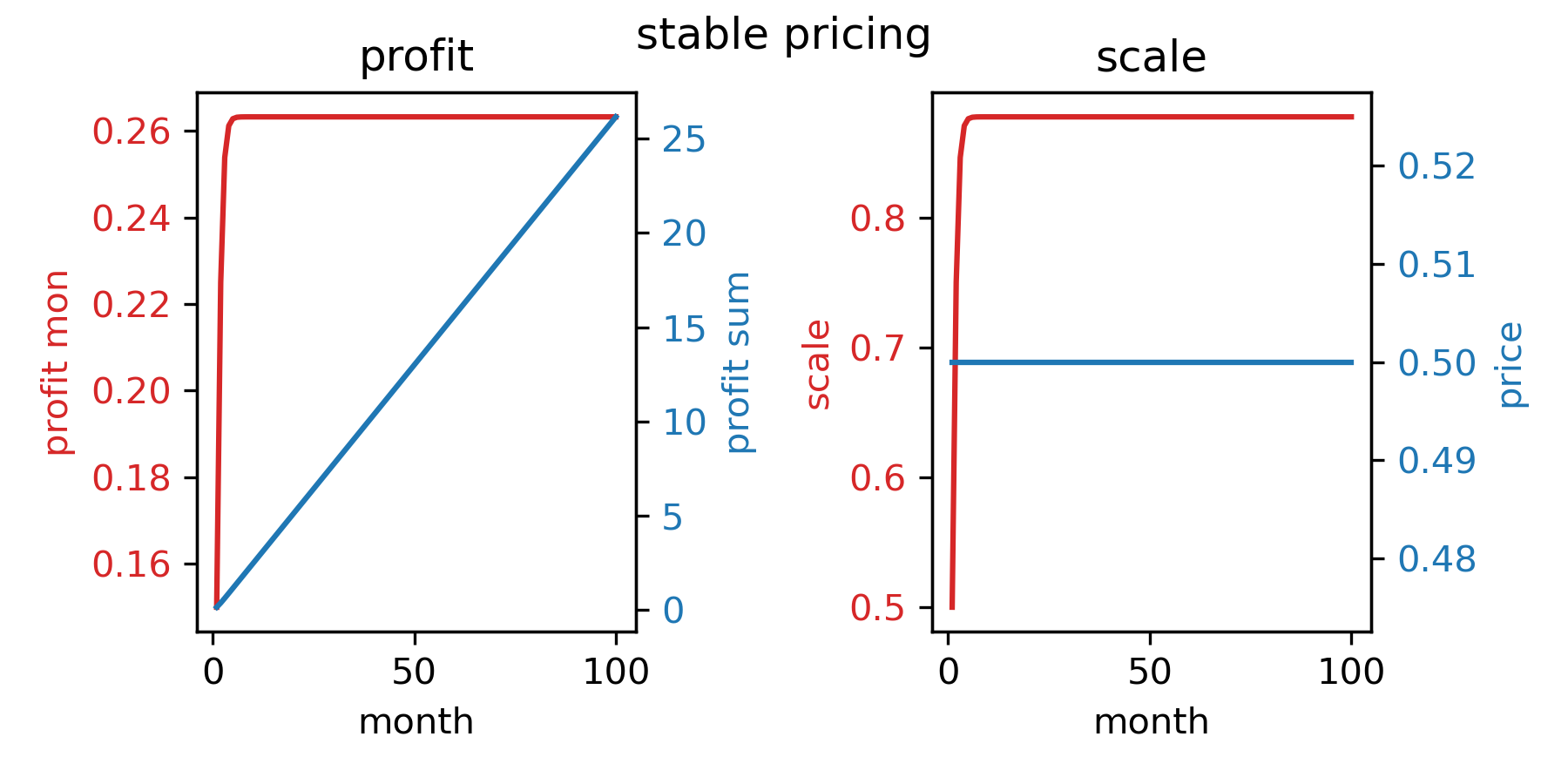
- 优势:当价格等于0.5时,市场的成长只有一个均衡点(即z^=z 与z^=g(z) 只有一个交点),市场可以自由地成长到这一点。在产品运营的前期,设定这一价格非常重要,它可以用以避免市场规模停滞在低位均衡。
- 改进之处:当产品运营进入中期,市场规模已经较大,过早陷入低位均衡的疑虑已经可以打消,价格可以做适当提升以提高利润(不过同时也应该防止提价过高掉回低位均衡)。
2.3.2、贪心策略
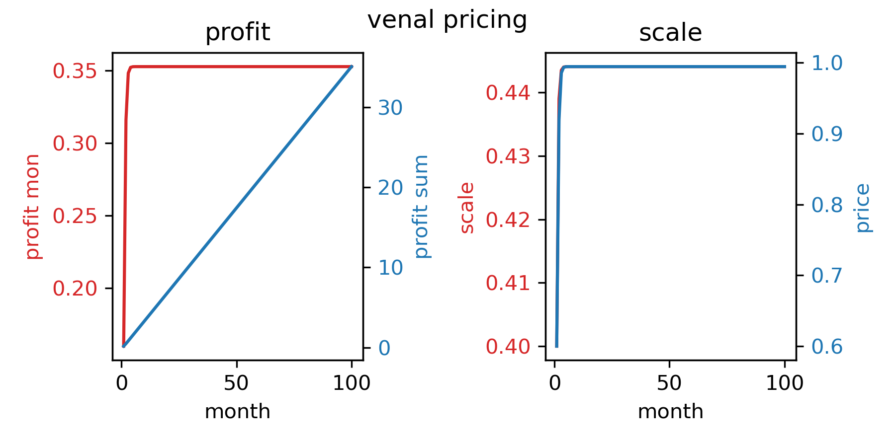
- 优势:能将每个月的利润最大化。
- 改进之处:由于短视地提价,实现了每个月的利润最大化却导致市场规模变小,陷入了低位均衡。
2.3.3、规模价格策略
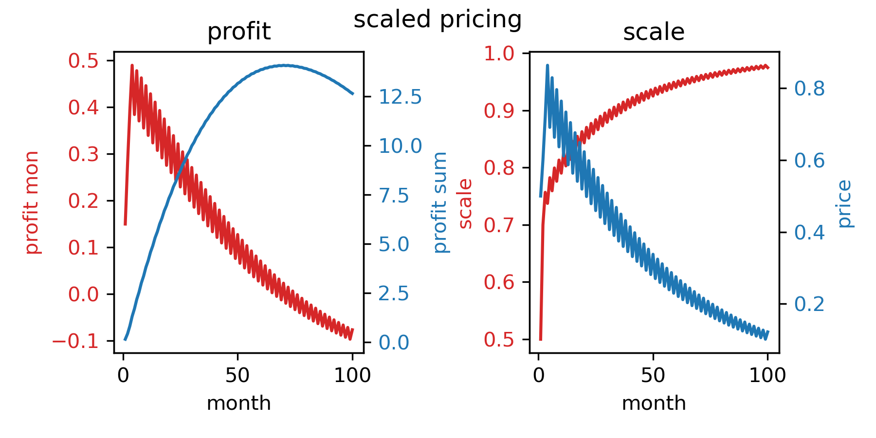
规模价格策略的表现最为糟糕。在市场规模扩大时,价格提高20%,这导致下月规模缩小,价格又降低20%,这又导致下月规模提高20,依次循环往复、来回震荡。一来一回,价格变为原先的96%,价格越降越低,最后甚至在做亏本买卖。
2.3.4、耐心策略和固定高价策略
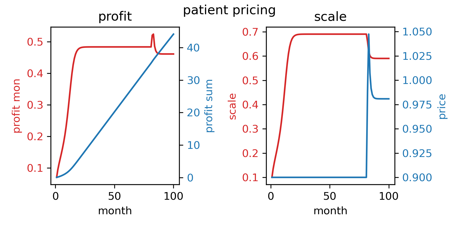
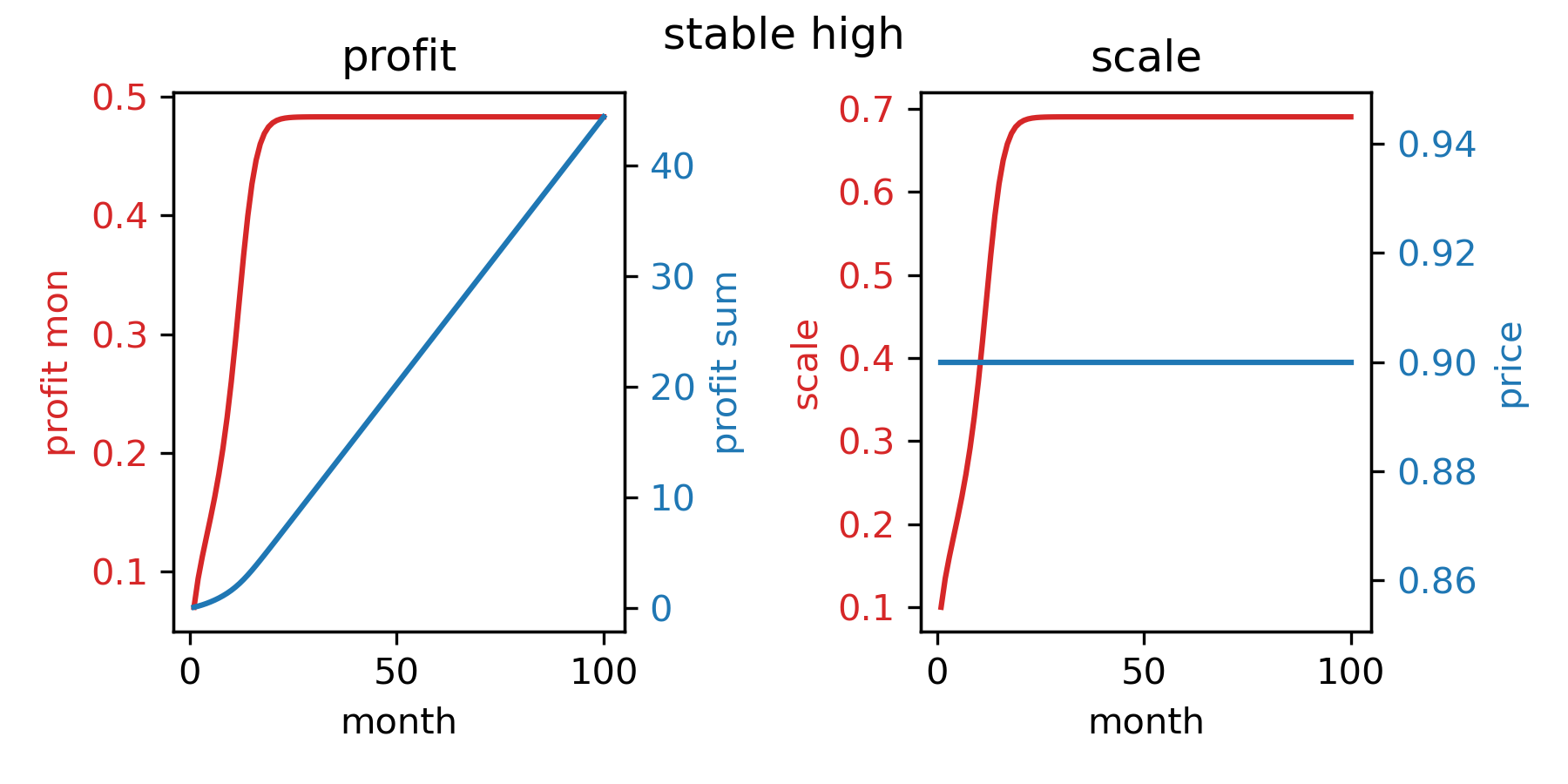
耐心策略的总利润比固定价格0.9更小,我们最大化次月利润来提价时,对利润的正向效果并不理想。而固定价格0.9之所以效果理想,是因为这时的均衡规模恰好接近最优均衡规模(见下一策略)。
2.3.5、均衡情况下的最佳定价策略
班上一位同学的定价策略最为成功。如果我们只考虑最终会把市场引向均衡的定价策略,那么存在一个最佳定价策略。他在数学上做出了证明。
根据均衡求解部分的等式(4),
均衡情况下有
均衡情况下,每月利润最大,总利润就最大。每月利润W可以表示为
W对z^ 求导,我们就可以得到,最大化W时,z^∗ ≈ 0.675, p∗≈0.918。
那么,第一轮的时候,我们只需要设置p1,以使
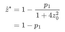
此时,p1≈0.325。这样,第二轮起,实际规模就达到了最优值 z^∗ 。
最后一轮,我们可以再调用贪心策略。不用顾忌未来的用户规模了,就可以最后再捞一把。
具体的代码如下:
def best(p0, z1, z2, rnd):
    if rnd == 1:
        return 0.325
    elif rnd == 100:
        return venal(p0, z1, z2, rnd)
    else:
        return 0.918
输出结果为:
模拟进行月数	10	20	30	40	50	60	70	80	90	100
best pricing	4.443	9.285	14.127	18.968	23.810	28.652	33.494	38.336	43.178	48.144
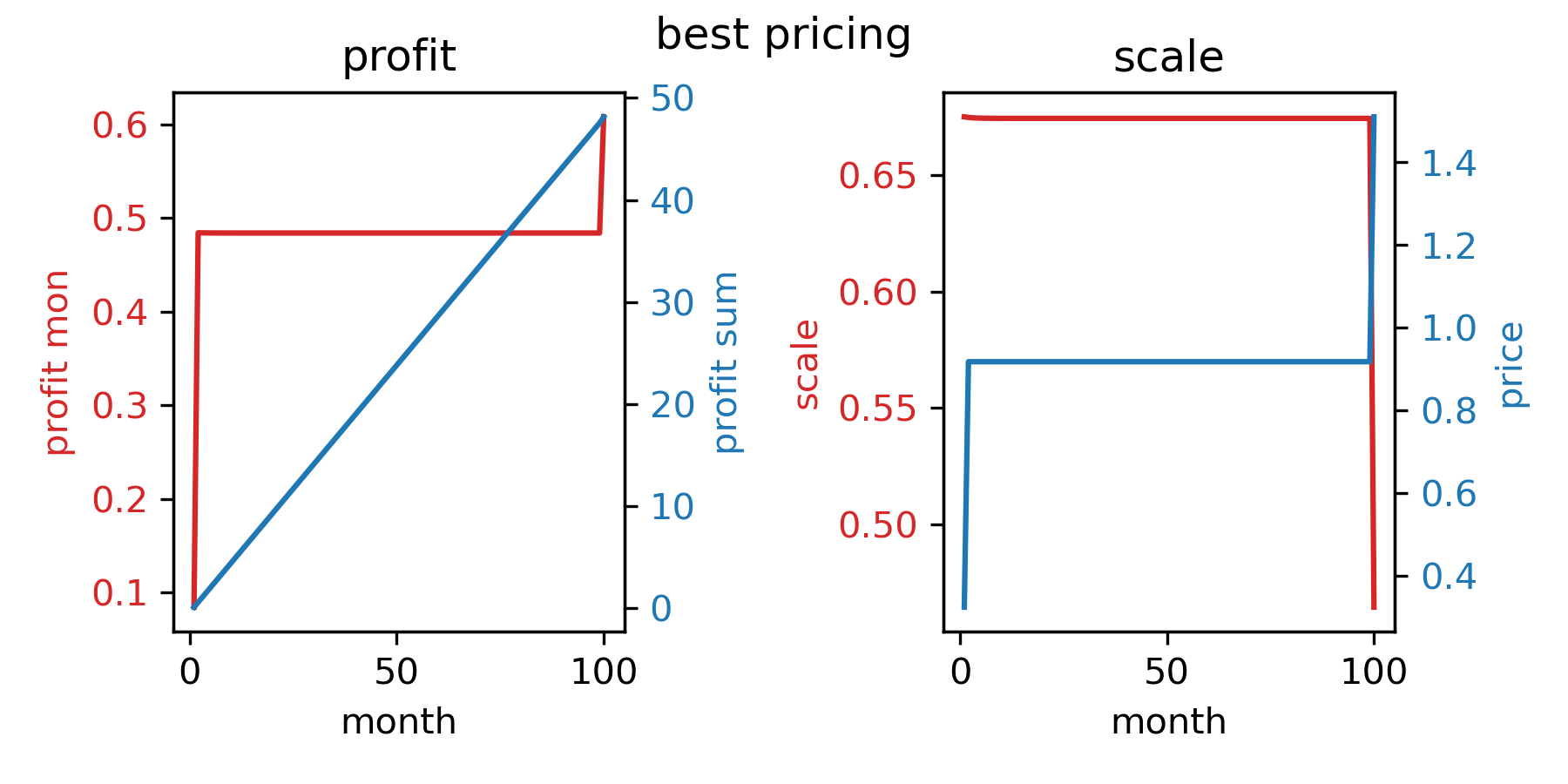
这一策略的总利润确实是最大的。
3、完整代码
import matplotlib.pyplot as plt
import numpy as np
from scipy.optimize import minimize_scalar


# compare different pricing strategies in a market with the network effect

class PriceFunc(object):
    def __init__(self, name, function, num):
        self.name = name
        self.function = function
        self.num = num

    def __str__(self):
        return self.name


def stable(p0, z1, z2, rnd):  # monthly prize stablized at 0.5
    return 0.5


def scaled(p0, z1, z2, rnd):  # if the scale increases, the price increases accordingly
    # p0: the price of last month
    # z1: the scale of the month before the last month
    # z2: the scale of the last month
    if z1 == None:
        return 0.5
    elif z1 < z2:
        return 1.2 * p0
    elif z1 > z2:
        return 0.8 * p0
    else:
        return p0


def venal(p0, z1, z2, rnd):  # designate the price to get the largest profit in this month
    k = 1 + 4 * z2 * z2
    # max((p - c) * x)
    # max((p-0.2) * (1 - p / k )
    # - p * p / k + ( 0.2 / k + 1 ) * p - 0.2 = 0
    # - 2 * p / k + (0.2 / k + 1) = 0
    # -2 * p + 0.2 + k = 0
    return 0.1 + k / 2


def stable_high(p0, z1, z2, rnd):
    return 0.9
    # When p = 25/27, g(z) and ˆz = z have only one point of contact and one point of intersection


def patient(p0, z1, z2, rnd):
    if z1 == None:
        return 0.9
    elif z2 > z1 and p0 == 0.9:
        return 0.9  # let the market grow
    elif z2 == z1 and p0 == 0.9:
        # I want to raise the price to gain more profit,
        # but I worry that a raise in price according to venal strategy will end with a large drop in scale
        # So I maximizing the profit of the month after the next month, instead of that of this month
        W = lambda p: -1 * (p - 0.2) * (1 - p / (1 + 4 * (1 - p / (1 + 4 * z2 * z2)) ** 2))
        res = minimize_scalar(W, bounds=(0, 5), method='bounded')
        return (res.x + p0) / 2
        # Market scale was stabilized by p = 0.9 at a high point in the last month, designate the mean to reduce the fluctuation
    else:
        W = lambda p: -1 * (p - 0.2) * (1 - p / (1 + 4 * (1 - p / (1 + 4 * z2 * z2)) ** 2))
        res = minimize_scalar(W, bounds=(0, 5), method='bounded')
        return res.x


def best(p0, z1, z2, rnd):
    if rnd == 1:
        return 0.325
    elif rnd == 100:
        return venal(p0, z1, z2, rnd)
    else:
        return 0.918


def profit_monthly(priceFunc):
    profit_sum = 0
    n = 0
    p = None
    z1 = None
    z2 = 0
    z_list = []
    p_list = []
    profit_mon_list = []
    profit_sum_list = []
    while True:
        n += 1
        p = priceFunc.function(p, z1, z2, n)  # price of this month
        p_list.append(p)
        z = 1 - p / (1 + 4 * z2 * z2)  # scale of this month
        z_list.append(z)
        profit_mon = (p - 0.2) * z
        profit_mon_list.append(profit_mon)
        profit_sum += profit_mon
        profit_sum_list.append(profit_sum)
        z1 = z2  # scale of the month before the last month
        z2 = z  # scale of the last month
        if n % 10 == 0:  # output the profit so far
            f.write('%.3f,' % profit_sum)
            print('%.3f' % profit_sum, end='\t')
        if n == 100:
            break
    f.write('\n')
    print()

    fig, (ax1, ax3) = plt.subplots(1, 2)
    fig.suptitle(priceFunc.name)
    ax1.set_title('profit')
    ax3.set_title('scale')
    # the graph of how monthly profit and profit sum change over time
    color1 = 'tab:red'
    color2 = 'tab:blue'
    xPoints = np.array(list(range(1, 101)))
    yPoints = np.array(profit_mon_list)
    ax1.plot(xPoints, yPoints, color=color1)
    ax1.set_xlabel('month')
    ax1.set_ylabel('profit mon', color=color1)
    ax1.tick_params(axis='y', labelcolor=color1)
    ax2 = ax1.twinx()
    ax2.set_ylabel('profit sum', color=color2)
    yPoints2 = np.array(profit_sum_list)
    ax2.plot(xPoints, yPoints2, color=color2)
    ax2.tick_params(axis='y', labelcolor=color2)
    # the graph of how the scale of the market and the price change over time
    yPoints3 = np.array(z_list)
    ax3.plot(xPoints, yPoints3, color=color1)
    ax3.set_xlabel('month')
    ax3.set_ylabel('scale', color=color1)
    ax3.tick_params(axis='y', labelcolor=color1)
    ax4 = ax3.twinx()
    ax4.set_ylabel('price', color=color2)
    yPoints4 = np.array(p_list)
    ax4.plot(xPoints, yPoints4, color=color2)
    ax4.tick_params(axis='y', labelcolor=color2)
    # fig.tight_layout()
    fig.set_size_inches(6, 3)
    fig.tight_layout()
    fig.savefig('./%i_%s.png' % (priceFunc.num, priceFunc.name), dpi=300)


# output the first row
f = open('./profit.csv', 'w', encoding='utf-8-sig')
f.write('模拟进行月数,')
print('模拟进行月数', end='\t')
for i in range(10, 101, 10):
    f.write('%i,' % i)
    print('%i' % i, end='\t')
f.write('\n')
print()

# the profit of each pricing strategy
funcList = [stable, scaled, venal, patient, stable_high, best]
titles = ['stable pricing', 'scaled pricing', 'venal pricing', 'patient pricing', 'stable high', 'best pricing']

for i in range(len(funcList)):
    priceFunc = PriceFunc(titles[i], funcList[i], i + 1)
    f.write('%s,' % titles[i])
    print('%s' % titles[i], end='\t')
    profit_monthly(priceFunc)

f.close()

