1、Multiple features
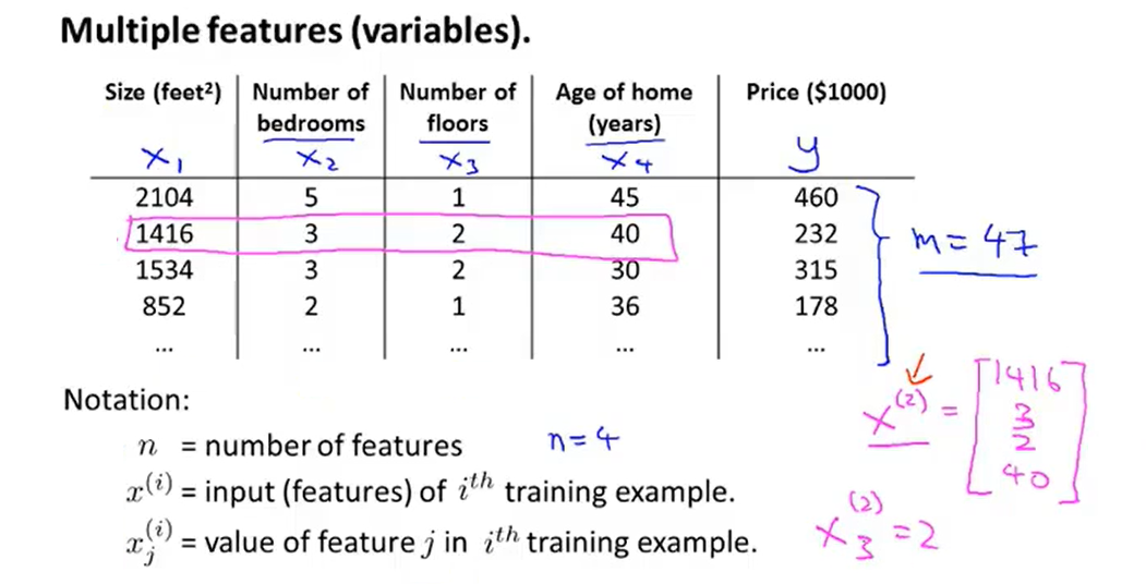
- So what the form of the hypothesis should be ?

- For convenience, define x0=1

- At this time, the parameter in the model is a (𝑛 + 1)-dimensional vector, and any training instance is also a (𝑛 + 1)-dimensional vector. The dimension of the feature matrix 𝑋 is {𝑚 ∗ (𝑛 + 1)} , so the formula can be simplified to :

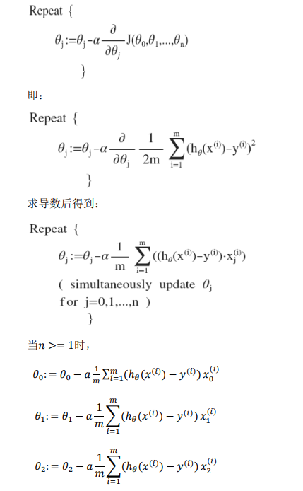
2、Gradient descent for multiple variables

- Here is the gradient descent looks like
def computeCost(X, y, theta):
 inner = np.power(((X * theta.T) - y), 2)
 return np.sum(inner) / (2 * len(X)
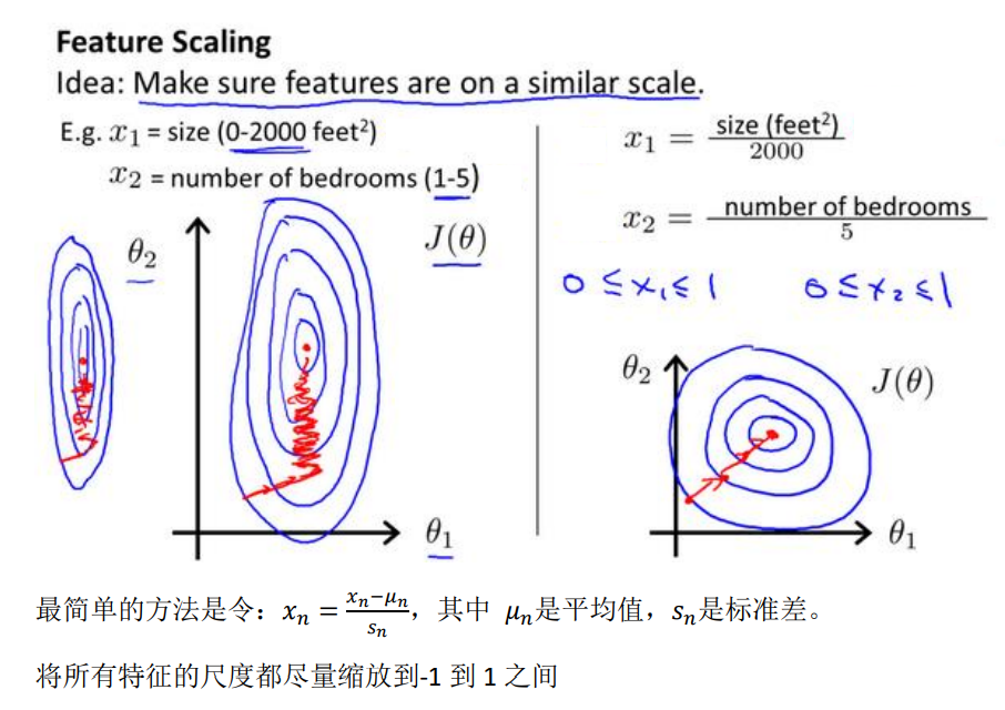
3、Gradient descent in practice I :Feature Scaling
- An idea about feature scaling(特征缩放) --- make sure features are on a similar scale and get every feature into approximately a -1≤xi≤1 range
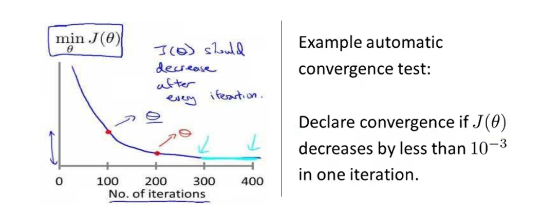
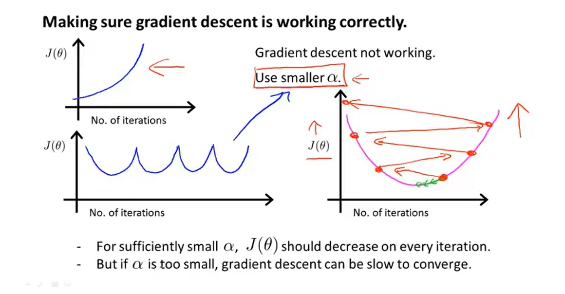
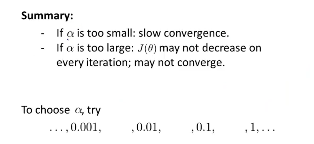
4、Gradient descent in practice II: Learning rate
5、Features and Polynomial Regression
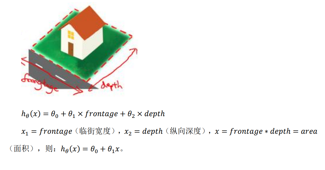
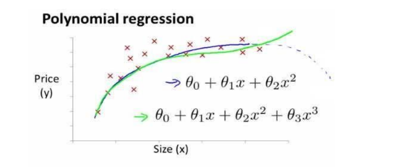
- Linear regression is not suitable for all data, sometimes we need a curve to fit our data, such as a quadratic model :


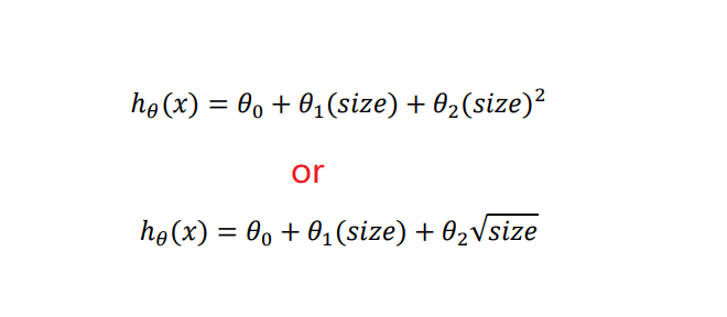
- According to the graphical characteristics of the function, we can also use :
6、Normal Equation
- Normal equation : method to solve for θ analytically
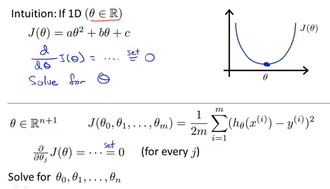
- It is too long and involved
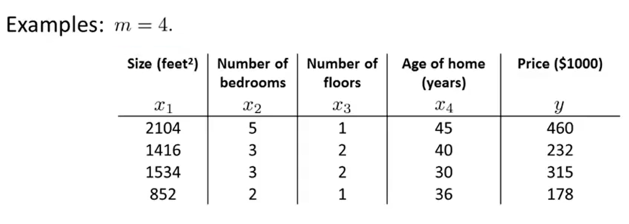
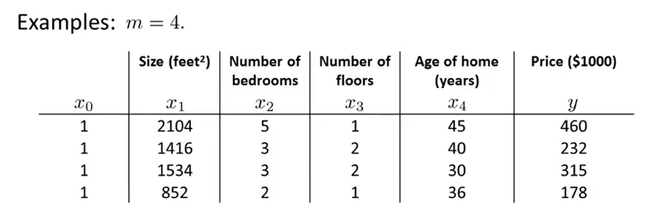
- And now,I am going to take the dataset and add an extra column
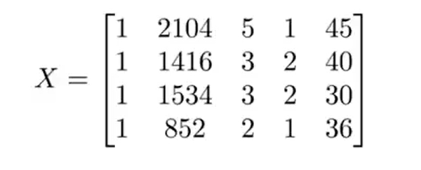
- Then construct a matrix X :
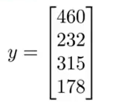
- And construct a vector y :
- Solve the vector using the normal equation :


pinv(X'*X)*X'*y
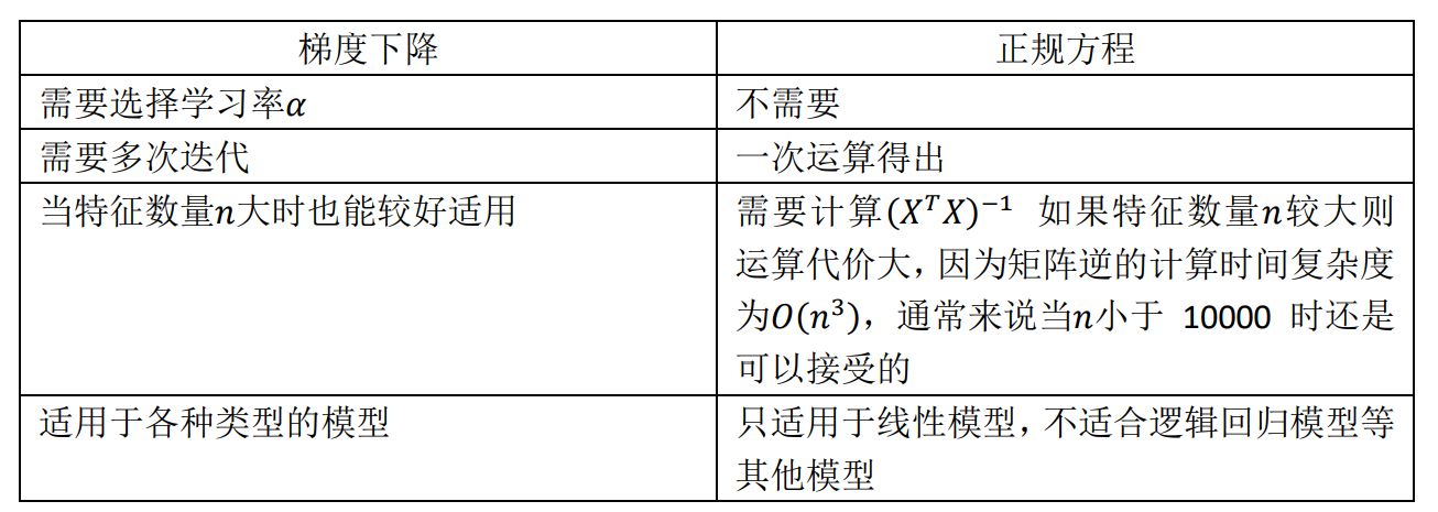
- How to choose gradient descent or normal equation ?
- Use python to implement Normal Equation
import numpy as np

def normalEqn(X, y):
 theta = np.linalg.inv(X.T@X)@X.T@y  #X.T@X 等价于 X.T.dot(X)
 return theta
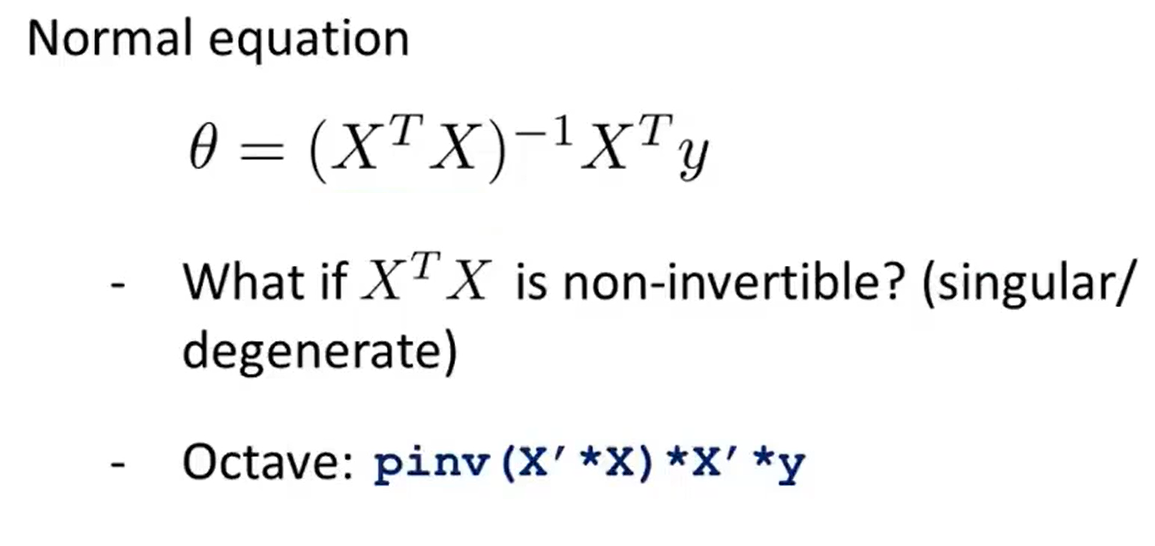
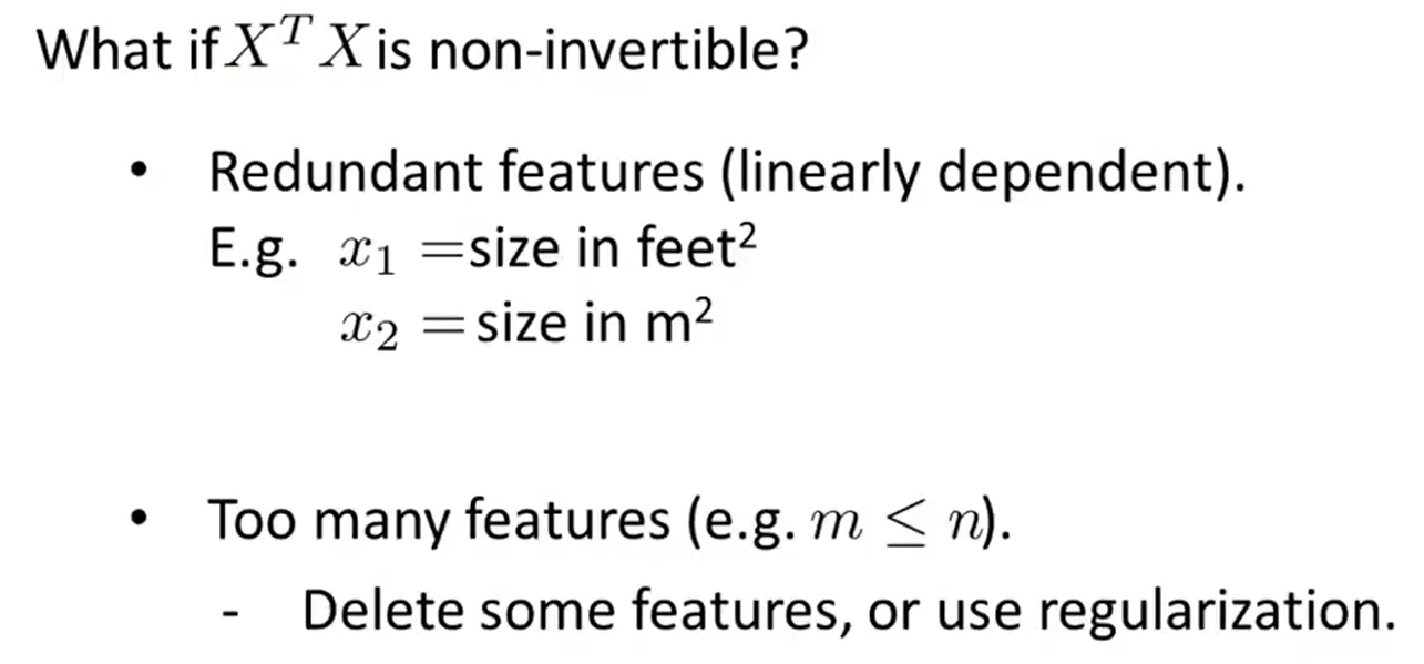
7、Normal Equation Non-invertibility
8、Supplement
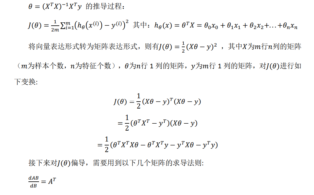
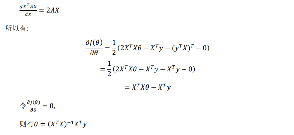


 多变量的线性回归内容
