python学习day-12 机器学习-监督学习-分类-支持向量机SVM&神经网络NN
一、SVM理论知识
1. 背景:
 两类?哪条线最好?


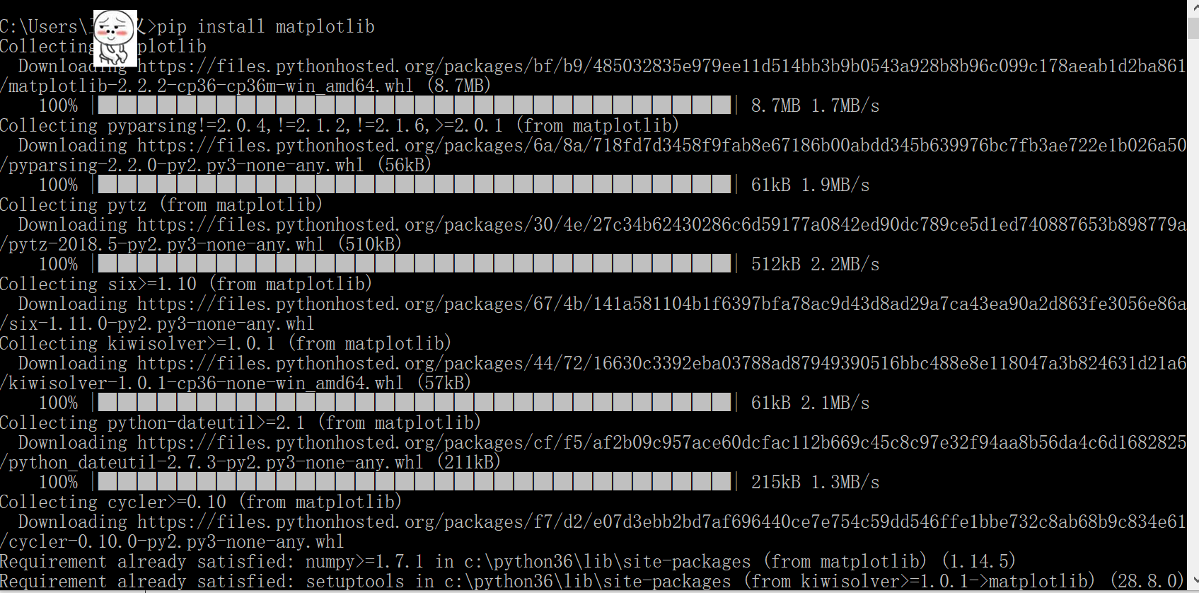
首先提到python绘图,matplotlib是不得不提的python最著名的绘图库,它里面包含了类似matlab的一整套绘图的API。因此,作为想要学*python绘图的童鞋们就得在自己的python环境中安装matplotlib库了,安装方式这里就不多讲,方法有很多,给个参考的。第二个代码里就需要调用绘图的库
1.线性不可分的理论知识


二、代码
1.简单代码
from sklearn import svm


x = [[2, 0], [1, 1], [2, 3]]
y = [0, 0, 1]
clf = svm.SVC(kernel = 'linear')
clf.fit(x, y)

print (clf)  #打印分类器  有很多参数

# get support vectors
print (clf.support_vectors_) #输出支持向量
# get indices of support vectors
print (clf.support_)  #输入的点,那几个点时支持向量对应的索引
# get number of support vectors for each class
print (clf.n_support_)
# print (clf.predict([2,0]..reshape))
# predictedY=clf.predict([2,0].reshape)
# print("predictedY:"+str(predictedY))
2.线性可分代码
import numpy as np
import pylab as pl
from sklearn import svm
# we create 40 separable points
X = np.r_[np.random.randn(20, 2) - [2, 2], np.random.randn(20, 2) + [2, 2]]
#利用随机函数产生点 二十个,二维,均值方差为2 -2在下方 2在上方
Y = [0]*20 +[1]*20 #前二十个点归类0,后二十点归类1
#fit the model建立模型
clf = svm.SVC(kernel='linear')
clf.fit(X, Y)
# get the separating hyperplane
w = clf.coef_[0]
a = -w[0]/w[1] #求斜率
xx = np.linspace(-5, 5)
yy = a*xx - (clf.intercept_[0])/w[1]
# plot the parallels to the separating hyperplane that pass through the support vectors
b = clf.support_vectors_[0]
yy_down = a*xx + (b[1] - a*b[0])
b = clf.support_vectors_[-1]
yy_up = a*xx + (b[1] - a*b[0])
print ("w: ", w)
print ("a: ", a)
# print "xx: ", xx
# print "yy: ", yy
print ("support_vectors_: ", clf.support_vectors_)
print ("clf.coef_: ", clf.coef_)
# switching to the generic n-dimensional parameterization of the hyperplan to the 2D-specific equation
# of a line y=a.x +b: the generic w_0x + w_1y +w_3=0 can be rewritten y = -(w_0/w_1) x + (w_3/w_1)
# plot the line, the points, and the nearest vectors to the plane
pl.plot(xx, yy, 'k-')
pl.plot(xx, yy_down, 'k--')
pl.plot(xx, yy_up, 'k--')
pl.scatter(clf.support_vectors_[:, 0], clf.support_vectors_[:, 1],
s=80, facecolors='none')
pl.scatter(X[:, 0], X[:, 1], c=Y, cmap=pl.cm.Paired)
pl.axis('tight')
pl.show()
3.线性不可分代码 人脸识别
from __future__ import print_function

from time import time
import logging  #需要打印一些进度
import matplotlib.pyplot as plt  #绘图

from sklearn.cross_validation import train_test_split
from sklearn.datasets import fetch_lfw_people
from sklearn.grid_search import GridSearchCV
from sklearn.metrics import classification_report
from sklearn.metrics import confusion_matrix
from sklearn.decomposition import RandomizedPCA
from sklearn.svm import SVC


print(__doc__)

# Display progress logs on stdout
logging.basicConfig(level=logging.INFO, format='%(asctime)s %(message)s')   #数据下载工作或者直接赋予图像


###############################################################################
# Download the data, if not already on disk and load it as numpy arrays

lfw_people = fetch_lfw_people(min_faces_per_person=70, resize=0.4)

# introspect the images arrays to find the shapes (for plotting)
n_samples, h, w = lfw_people.images.shape

# for machine learning we use the 2 data directly (as relative pixel
# positions info is ignored by this model)
X = lfw_people.data
n_features = X.shape[1]    #每个特征向量的维度,返回行数列数

# the label to predict is the id of the person
y = lfw_people.target
target_names = lfw_people.target_names
n_classes = target_names.shape[0]

print("Total dataset size:")
print("n_samples: %d" % n_samples)
print("n_features: %d" % n_features)
print("n_classes: %d" % n_classes)


###############################################################################
# Split into a training set and a test set using a stratified k fold

# split into a training and testing set
X_train, X_test, y_train, y_test = train_test_split(
    X, y, test_size=0.25)


###############################################################################
# Compute a PCA (eigenfaces) on the face dataset (treated as unlabeled
# dataset): unsupervised feature extraction / dimensionality reduction
n_components = 150

print("Extracting the top %d eigenfaces from %d faces"
      % (n_components, X_train.shape[0]))
t0 = time()
pca = RandomizedPCA(n_components=n_components, whiten=True).fit(X_train)    #PCA降维
print("done in %0.3fs" % (time() - t0))

eigenfaces = pca.components_.reshape((n_components, h, w))

print("Projecting the input data on the eigenfaces orthonormal basis")
t0 = time()
X_train_pca = pca.transform(X_train)
X_test_pca = pca.transform(X_test)
print("done in %0.3fs" % (time() - t0))


###############################################################################
# Train a SVM classification model

print("Fitting the classifier to the training set")
t0 = time()
param_grid = {'C': [1e3, 5e3, 1e4, 5e4, 1e5],
              'gamma': [0.0001, 0.0005, 0.001, 0.005, 0.01, 0.1], }
clf = GridSearchCV(SVC(kernel='rbf', class_weight='auto'), param_grid)
clf = clf.fit(X_train_pca, y_train)
print("done in %0.3fs" % (time() - t0))
print("Best estimator found by grid search:")
print(clf.best_estimator_)


###############################################################################
# Quantitative evaluation of the model quality on the test set

print("Predicting people's names on the test set")
t0 = time()
y_pred = clf.predict(X_test_pca)
print("done in %0.3fs" % (time() - t0))

print(classification_report(y_test, y_pred, target_names=target_names))
print(confusion_matrix(y_test, y_pred, labels=range(n_classes)))


###############################################################################
# Qualitative evaluation of the predictions using matplotlib

def plot_gallery(images, titles, h, w, n_row=3, n_col=4):
    """Helper function to plot a gallery of portraits"""
    plt.figure(figsize=(1.8 * n_col, 2.4 * n_row))
    plt.subplots_adjust(bottom=0, left=.01, right=.99, top=.90, hspace=.35)
    for i in range(n_row * n_col):
        plt.subplot(n_row, n_col, i + 1)
        plt.imshow(images[i].reshape((h, w)), cmap=plt.cm.gray)
        plt.title(titles[i], size=12)
        plt.xticks(())
        plt.yticks(())


# plot the result of the prediction on a portion of the test set

def title(y_pred, y_test, target_names, i):
    pred_name = target_names[y_pred[i]].rsplit(' ', 1)[-1]
    true_name = target_names[y_test[i]].rsplit(' ', 1)[-1]
    return 'predicted: %s\ntrue:      %s' % (pred_name, true_name)

prediction_titles = [title(y_pred, y_test, target_names, i)
                     for i in range(y_pred.shape[0])]

plot_gallery(X_test, prediction_titles, h, w)

# plot the gallery of the most significative eigenfaces

eigenface_titles = ["eigenface %d" % i for i in range(eigenfaces.shape[0])]
plot_gallery(eigenfaces, eigenface_titles, h, w)

plt.show()


二、神经网络算法
1. 背景:


![]() 导数:
导数:![]()
![]() 导数:
导数:![]()
 导数:
导数:

导数:
导数:8.运行程序遇到了问题
Python提示AttributeError 或者DeprecationWarning: This module was deprecated解决方法
在使用Python的sklearn库时,发现sklearn的cross_validation不能使用,在pycharm上直接显示为被横线划掉。
运行程序

解决方法就是把
from sklearn.cross_validation import train_test_split
改为:
from sklearn.model_selection import train_test_split

二、代码部分
1、基础代码------编写原始代码
import numpy as np
#定义了两个函数和他们对应的导数
def tanh(x):
    return np.tanh(x)

def tanh_deriv(x):
    return 1.0 - np.tanh(x)*np.tanh(x)

def logistic(x):
    return 1/(1 + np.exp(-x))

def logistic_derivative(x):
    return logistic(x)*(1-logistic(x))

#定义一个类
class NeuralNetwork:
    def __init__(self, layers, activation='tanh'):
        """
        :param layers: A list containing the number of units in each layer.
        Should be at least two values
        :param activation: The activation function to be used. Can be
        "logistic" or "tanh"
        """
        if activation == 'logistic':
            self.activation = logistic
            self.activation_deriv = logistic_derivative
        elif activation == 'tanh':
            self.activation = tanh
            self.activation_deriv = tanh_deriv

        self.weights = []  #每两个有一个权重,所以要初始化一个权重
        for i in range(1, len(layers) - 1):  #除了输出层,我们都要给他赋予一个随机的权重,从第二层开始
            self.weights.append((2*np.random.random((layers[i - 1] + 1, layers[i] + 1))-1)*0.25)  #-0.25到+0.25之间的
            self.weights.append((2*np.random.random((layers[i] + 1, layers[i + 1]))-1)*0.25)
    #定义一个训练方法
    def fit(self, X, y, learning_rate=0.2, epochs=10000):   #learning_rate 代表l   epoches定义循环抽样的次数
        X = np.atleast_2d(X)  #要确定输入的值至少一个一个2d的值
        temp = np.ones([X.shape[0], X.shape[1]+1]) #shape会返回x的行数和列数。   .shape[0]:返回的就是行数   就得到一个与x行数相同,列数大x一个
        temp[:, 0:-1] = X  # adding the bias unit to the input layer
        X = temp
        y = np.array(y)

        for k in range(epochs):
            i = np.random.randint(X.shape[0])
            a = [X[i]]

            for l in range(len(self.weights)):  #going forward network, for each layer
                a.append(self.activation(np.dot(a[l], self.weights[l])))  #Computer the node value for each layer (O_i) using activation function
            error = y[i] - a[-1]  #Computer the error at the top layer
            deltas = [error * self.activation_deriv(a[-1])] #For output layer, Err calculation (delta is updated error)

            #Staring backprobagation
            for l in range(len(a) - 2, 0, -1): # we need to begin at the second to last layer
                #Compute the updated error (i,e, deltas) for each node going from top layer to input layer

                deltas.append(deltas[-1].dot(self.weights[l].T)*self.activation_deriv(a[l]))
            deltas.reverse()
            for i in range(len(self.weights)):
                layer = np.atleast_2d(a[i])
                delta = np.atleast_2d(deltas[i])
                self.weights[i] += learning_rate * layer.T.dot(delta)

    def predict(self, x):
        x = np.array(x)
        temp = np.ones(x.shape[0]+1)
        temp[0:-1] = x
        a = temp
        for l in range(0, len(self.weights)):
            a = self.activation(np.dot(a, self.weights[l]))
        return a
2、简单应用
from NeuralNetwork import NeuralNetwork
import numpy as np

nn = NeuralNetwork([2, 2, 1], 'tanh')  #第一个参数对应是有几层,每一层对应的个数,   第二个代表了activation function
X = np.array([[0, 0], [0, 1], [1, 0], [1, 1]])
y = np.array([0, 1, 1, 0])
nn.fit(X, y)
for i in [[0, 0], [0, 1], [1, 0], [1, 1]]:
    print(i, nn.predict(i))
3、手写数字识别分类
#!/usr/bin/python
# -*- coding:utf-8 -*-

# 每个图片8x8  识别数字:0,1,2,3,4,5,6,7,8,9

import numpy as np
from sklearn.datasets import load_digits
from sklearn.metrics import confusion_matrix, classification_report
from sklearn.preprocessing import LabelBinarizer
from NeuralNetwork import NeuralNetwork
# from sklearn.cross_validation import train_test_split
from sklearn.model_selection import train_test_split

digits = load_digits() #装载数据
X = digits.data
y = digits.target
X -= X.min()  # normalize the values to bring them into the range 0-1  预处理
X /= X.max()

nn = NeuralNetwork([64, 100, 10], 'logistic')
X_train, X_test, y_train, y_test = train_test_split(X, y)
labels_train = LabelBinarizer().fit_transform(y_train)
labels_test = LabelBinarizer().fit_transform(y_test)
print ("start fitting")
nn.fit(X_train, labels_train, epochs=3000)
predictions = []
for i in range(X_test.shape[0]):
    o = nn.predict(X_test[i])
    predictions.append(np.argmax(o))
print (confusion_matrix(y_test, predictions))  #坐落在对角线上的代表了预测对了
print (classification_report(y_test, predictions))  #

 浙公网安备 33010602011771号