（转）Markov Chain Monte Carlo

Nice R Code

Punning code better since 2013

• RSS

• Blog
• Archives
• Guides
• Modules
• About

Markov Chain Monte Carlo

10 JUNE 2013

This topic doesn’t have much to do with nicer code, but there is probably some overlap in interest. However, some of the topics that we cover arise naturally here, so read on! We’ll flesh out sections that use interesting programming techniques (especially higher order functions) over time.

What is MCMC and when would you use it?

MCMC is simply an algorithm for sampling from a distribution.

It’s only one of many algorithms for doing so. The term stands for “Markov Chain Monte Carlo”, because it is a type of “Monte Carlo” (i.e., a random) method that uses “Markov chains” (we’ll discuss these later). MCMC is just one type of Monte Carlo method, although it is possible to view many other commonly used methods as simply special cases of MCMC.

As the above paragraph shows, there is a bootstrapping problem with this topic, that we will slowly resolve.

Why would I want to sample from a distribution?

You may not realise you want to (and really, you may not actually want to). However, sampling from a distribution turns out to be the easiest way of solving some problems. In MCMC’s use in statistics, sampling from a distribution is simply a means to an end.

Probably the most common way that MCMC is used is to draw samples from the posterior probability distribution of some model in Bayesian inference. With these samples, you can then ask things like “what is the mean and credibility interval for a parameter?”.

For example, suppose that you have fit a model where the posterior probability density is some function $f$ of parameters $(x, y)$. Then, to compute the mean value of parameter $x$, you would compute

which you can read simply as “the value of $x$ multiplied by the probability of parameters $(x, y)$, integrated over all possible values that $x$ and $y$ could take.

An alternative way to compute this value is simulate $k$ observations, $[(x,y)^{(1)}, \ldots, (x,y)^{(k)}]$, from $f(x,y)$ and compute the sample mean as

where $x^{(j)}$ is the the $x$ value from the $j$th sample.

If these samples are independent samples from the distribution, then as $k \to \infty$ the estimated mean of $x$ will converge on the true mean.

Suppose that our target distribution is a normal distribution with mean m and standard deviation s. Obviously the mean of this distribution is m, but let’s try to show that by drawing samples from the distribution.

As an example, consider estimating the mean of a normal distribution with mean m and standard deviation s (here, I’m just going to use parameters corresponding to a standard normal):

1 2	m <- 0 s <- 1

We can easily sample from this distribution using the rnorm function:

1 2	set.seed(1) samples <- rnorm(10000, m, s)

The mean of the samples is very close to the true mean (zero):

1	mean(samples)

1	## [1] -0.006537

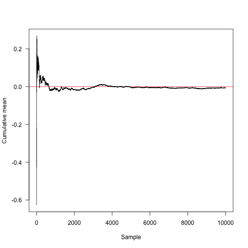
In fact, in this case, the expected variance of the estimate with $n$ samples is $1/n$, so we’d expect most values to lie within $\pm 2\, / \sqrt{n} = 0.02$ of the true mean for 10,000 points.

1	summary(replicate(1000, mean(rnorm(10000, m, s))))

1 2	## Min. 1st Qu. Median Mean 3rd Qu. Max. ## -0.03250 -0.00580 0.00046 0.00042 0.00673 0.03550

This function computes the cumulative mean (that is, for element $k$, the sum of elements $1, 2, \ldots, k$ divided by $k$).

1 2	cummean <- function(x) cumsum(x) / seq_along(x)

Here is the convergence towards the true mean (red line at 0).

1 2	plot(cummean(samples), type="l", xlab="Sample", ylab="Cumulative mean", panel.first=abline(h=0, col="red"), las=1)

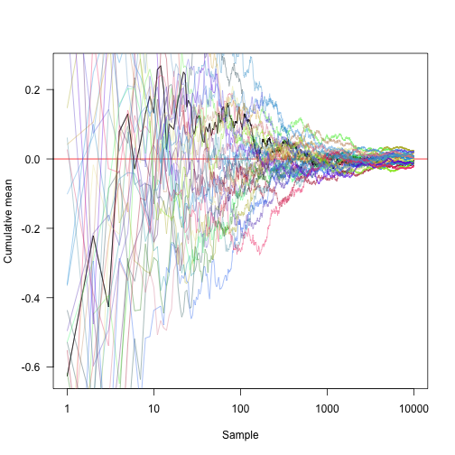
Transforming the x axis onto a log scale and showing another 30 random approaches:

1 2 3 4 5 6

set.seed(1) plot(cummean(samples), type="l", xlab="Sample", ylab="Cumulative mean", panel.first=abline(h=0, col="red"), las=1, log="x") for (i in seq_len(30)) lines(cummean(rnorm(10000, m, s)), col=rgb(runif(1), runif(1), runif(1), .5))

How does this work? Consider the integral

If this can be decomposed into the product of a function $f(x)$ and a probability density function $p(x)$, then

Note that the right hand side is simply the expectation $E[f(x)]$. By the Law of Large Numbers, the expected value is the limit of the sample mean as the sample size grows to infinity. So we can approximate $E[f(x)]$ as

You can do lots of similar things with this approach. For example, if you want to draw a 95\% credibility interval around the estimate $\bar x$, you could estimate the bottom component of that by solving

for $a$. Or, you can just take the sample quantile from your series of sampled points.

This is the analytically computed point where 2.5\% of the probability density is below:

1 2 3

p <- 0.025 a.true <- qnorm(p, m, s) a.true

1	## [1] -1.96

We can estimate this by direct integration in this case (using the argument above)

1 2 3 4 5

f <- function(x) dnorm(x, m, s) g <- function(a) integrate(f, -Inf, a)$value a.int <- uniroot(function(x) g(x) - p, c(-10, 0))$root a.int

1	## [1] -1.96

And estimate the point by Monte Carlo integration:

1 2	a.mc <- unname(quantile(samples, p)) a.mc

1	## [1] -2.023

Note that this has an error around it:

1	a.true - a.mc

1	## [1] 0.06329

But in the limit as the sample size goes to infinity, this will converge. Furthermore, it is possible to make statements about the nature of the error; if we repeat sampling process 100 times, we get a series of estimate that have error on around the same order of magnitide as the error around the mean:

1 2	a.mc <- replicate(100, quantile(rnorm(10000, m, s), p)) summary(a.true - a.mc)

1 2	## Min. 1st Qu. Median Mean 3rd Qu. Max. ## -0.05840 -0.01640 -0.00572 -0.00024 0.01400 0.07880

Still not convinced?

This sort of thing is really common. In most Bayesian inference you have a posterior distribution that is a function of some (potentially large) vector of parameters and you want to make inferences about a subset of these parameters. In a heirarchical model, you might have a large number of random effect terms being fitted, but you mostly want to make inferences about one parameter. In a Bayesian framework you would compute the marginal distribution of your parameter of interest over all the other parameters (this is what we were trying to do above). If you have 50 other parameters, this is a really hard integral!

To see why this is hard, consider the region of parameter space that contains “interesting” parameter values: that is, parameter values that have probabilities that are appreciably greater than zero (these are the only regions that contribute meaningfully to the integrals that we’re interested in, so if we spend our time doing a grid search and mostly hitting zeros then we’ll be wasting time).

For an illustration of the problem,

• consider a circle of radius $r$ within a square with sides of length $2r$; the “interesting” region of space is $\pi r^2 / 4 r^2 = \pi / 4$, so we’d have a good chance that a randomly selected point lies within the circle.
• For a sphere with radius $r$ in a cube with sides of length $2r$, the volume of the sphere is $4/(3 \pi r^3)$ and the volume of the cube is $(2d)^3$, so $4/3 \pi / 8 \approx 52\%$ of the volume is “interesting”
• As the dimensionality of the problem, $d$, increases (using a hypersphere in a hypercube) this ratio is

1 2 3 4

d <- 2:10 plot(d, pi^(d/2) / (d * 2^(d-1) * gamma(d/2)), log="y", las=1, xlab="Dimension", ylab="Proportion of hypercube filled with hypersphere")

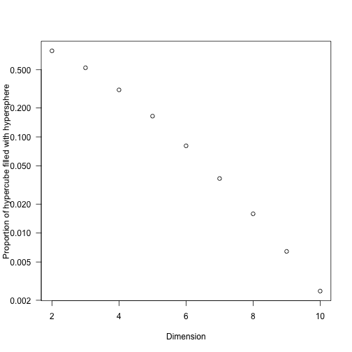
So we don’t need to add many dimensions to be primarily interested in a very small fraction of the potential space. (It’s also worth remembering that most integrals that converge must be zero almost everywhere or have a naturally very constrained domain.)

As a less abstract idea, consider a multivariate normal distribution with zero covariance terms, a mean at the origin, and unit variances. These have a distinct mode (maximum) at the origin, and the ratio of probabilities at a point and at the mode is

The thing about this function is that any large value of $x_i$ will cause the probability to be low. So as the dimension of the problem increases, the interesting space gets very small. Consider sampling within the region $-5 < x_i < 5$, and count how many of 10,000 sampled points have a relative probability greater than 1/1000

1 2 3 4 5 6 7

test <- function(d, x=5) exp(-sum(runif(d, -x, x)^2)) > 1/1000 f <- function(d, n) mean(replicate(n, test(d))) d <- 1:10 data.frame(dimension=d, p.interesting=sapply(d, f, 10000))

1 2 3 4 5 6 7 8 9 10 11

## dimension p.interesting ## 1 1 0.5219 ## 2 2 0.2173 ## 3 3 0.0739 ## 4 4 0.0218 ## 5 5 0.0070 ## 6 6 0.0025 ## 7 7 0.0006 ## 8 8 0.0000 ## 9 9 0.0000 ## 10 10 0.0000

which drops off much like the hypersphere case. Even by looking at only 4-5 dimensions we’re likely to waste a lot of time if we tried to exhaustively integrate over parameter space.

Why doesn’t “normal statistics” use Monte Carlo methods?

For many problems in traditionally taught statistics, rather than sampling from a distribution you maximise or maximise a function. So we’d take some function that describes the likelihood and maximise it (maximum likelihood inference), or some function that computes the sum of squares and minimise it.

The reasons for this difference are a little subtle, but boil down to whether or not you feel that you could possibly put a probability distribution over a parameter – is it something you could sample? Fisher in particular had strong thoughts on this, thoughts which are argued more recently by AWF Edwards in the book “Likelihood”. To avoid having to sample from a distribution (or really, to avoid the idea that one could draw samples from a probability distribution of parameters), error estimates in frequentist statistics tend to either be asymptotic large-data estimates or perhaps based on the bootstrap.

However, the role played by Monte Carlo methods in Bayesian statistics is the same as the optimisation routine in frequentist statistics; it’s simply the algorithm for doing the inference. So once you know basically what MCMC is doing, you can treat it like a black box in the same way that most people treat their optimisation routines as a black box.

Markov Chain Monte Carlo

At this point, suppose that there is some target distribution that we’d like to sample from, but that we cannot just draw independent samples from like we did before. There is a solution for doing this using the Markov Chain Monte Carlo (MCMC). First, we have to define some things so that the next sentence makes sense:What we’re going to do is try to construct a Markov chain that has our hard-to-sample-from target distribution as its stationary distribution.

Definitions

Let $X_t$ denote the value of some random variable at time $t$. A Markov chain generates a series of samples $[X0, X1, X2, \ldots, Xt]$ by starting at some point $X_0$, and then following a series of stochastic steps.

Markov chains satisfy the Markov property. The Markov property is the stochastic process version of “what happens in Vegas stays in Vegas”; basically it doesn’t matter how you got to some state $x$, the probability of transition out of $x$ is unchanged, or:

The transition from one step to the next is described by the transition kernel, which can be described by the probability (or for continuous variables the probability density) of a transition from state $i$ to state $j$ as

Let $\pi_j(t) = \Pr(X_t = s_j)$ be the probability that the chain is in state $j$ at time (step) $t$, and define $\vec\pi(t)$ be the vector of probabilites over possible states. Then, given $\vec\pi(t)$, we can compute $\vec\pi(t+1)$ using the Chapman-Kolmogorov equation.

that is; the probability that we were in state $k$ multiplied by the probability of making the transition from $k$ to $i$, summed over all possible source states $k$. Using the book-keeping of linear algebra, let $\mathbf{P}$ be the probability transition matrix – the matrix whose $i,j$th element is $P(i \to j)$, and rewrite the above equation as

Note that we can iterate this equation easily:

$$ \vec\pi(t+2) = \vec\pi(t+1)\mathbf{P} $$ $$ \vec\pi(t+2) = \vec\pi(t)\mathbf{P}\mathbf{P} $$ $$ \vec\pi(t+2) = \vec\pi(t)\mathbf{P}^2 $$

Stationary distributions

If there is some vector $\vec\pi^*$ that satisfies

then $\vec\pi^$ is the *stationary distribution of this Markov chain. Intuitively, think of this as the eventual characteristic set of states that the system will set in to; run for long enough that the system has “forgotten” its initial state, then the $i$th element of this vector is the probability that the system will be in state $i$.

The Markov chain will have a stationary distribution if the process is irreducible (every state is visitable from every other state) and aperiodic (the number of steps between two visits of a state is not a fixed integer multiple number of steps).

Mathematically, $\vec\pi^*$ is the left eigenvector assicated with the eigenvalue = 1.

Here’s a quick definition to make things more concrete (but note that this has nothing to do with MCMC itself – this is just to think about Markov chains!). Suppose that we have a three-state Markov process. Let P be the transition probability matrix for the chain:

1 2 3 4

P <- rbind(c(.5, .25, .25), c(.2, .1, .7), c(.25, .25, .5)) P

1 2 3 4

## [,1] [,2] [,3] ## [1,] 0.50 0.25 0.25 ## [2,] 0.20 0.10 0.70 ## [3,] 0.25 0.25 0.50

note that the rows of P sum to one:

1	rowSums(P)

1	## [1] 1 1 1

This can be interpreted as saying that we must go somewhere, even if that place is the same place. The entry P[i,j] gives the probability of moving from state i to state j (so this is the $P(i\to j)$ mentioned above.

Note that unlike the rows, the columns do not necessarily sum to 1:

1	colSums(P)

1	## [1] 0.95 0.60 1.45

This function takes a state vector x (where x[i] is the probability of being in state i) and iterates it by multiplying by the transition matrix P, advancing the system for n steps.

1 2 3 4 5 6 7

iterate.P <- function(x, P, n) { res <- matrix(NA, n+1, length(x)) res[1,] <- x for (i in seq_len(n)) res[i+1,] <- x <- x %*% P res }

Starting with the system in state 1 (so x is the vector $[1,0,0]$ indicating that there is a 100\% probability of being in state 1 and no chance of being in any other state), and iterating for 10 steps:

1 2	n <- 10 y1 <- iterate.P(c(1, 0, 0), P, n)

Similarly, for the other two possible starting states:

1 2	y2 <- iterate.P(c(0, 1, 0), P, n) y3 <- iterate.P(c(0, 0, 1), P, n)

This shows the convergence on the stationary distribution.

1 2 3

matplot(0:n, y1, type="l", lty=1, xlab="Step", ylab="y", las=1) matlines(0:n, y2, lty=2) matlines(0:n, y3, lty=3)

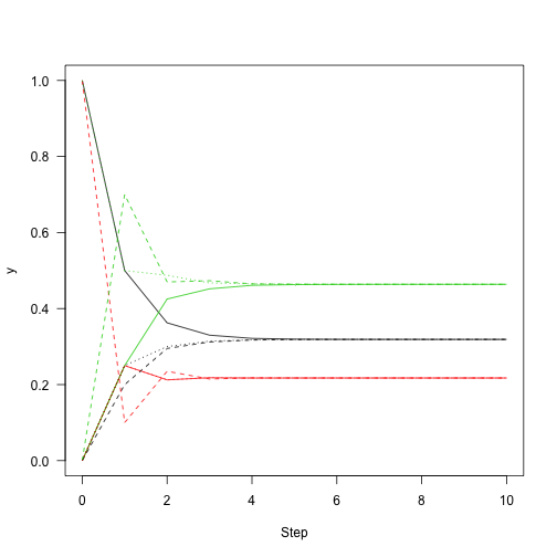
which means that regardless of the starting distribution, there is a 32\% chance of the chain being in state 1 after about 10 or more iterations regardless of where it started. So, knowing about the state of this chain at one point in time gives you information about where it is likely to be for only a few steps.

We can use R’s eigen function to extract the leading eigenvector for the syste (the t() here transposes the matrix so that we get the left eigenvector).

1 2	v <- eigen(t(P), FALSE)$vectors[,1] v <- v/sum(v) # normalise eigenvector

Then add points to the figure from before showing how close we are to convergence:

1 2 3 4

matplot(0:n, y1, type="l", lty=1, xlab="Step", ylab="y", las=1) matlines(0:n, y2, lty=2) matlines(0:n, y3, lty=3) points(rep(10, 3), v, col=1:3)

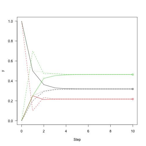
Following the definition of eigenvectors, multiplying the eigenvector by the transition matrix returns the eigenvector itself:

1	drop(v %*% P) - v

1	## [1] -1.110e-16 1.388e-16 0.000e+00

(strictly, this should be the eigenvalue multiplied by v, but the leading eigenvalue is always 1 for these matrices).

The proceedure above iterated the overall probabilities of different states; not the actual transitions through the system. So, let’s iterate the system, rather than the probability vector. The function run here takes a state (this time, just an integer indicating which of the states $1, 2, 3$ the system is in), the same transition matrix as above, and a number of steps to run. Each step, it looks at the possible places that it could transition to and chooses 1 (this uses R’s sample function).

1 2 3 4 5 6

run <- function(i, P, n) { res <- integer(n) for (t in seq_len(n)) res[[t]] <- i <- sample(nrow(P), 1, pr=P[i,]) res }

Here’s the chain running around for 100 steps:

1 2	samples <- run(1, P, 100) plot(samples, type="s", xlab="Step", ylab="State", las=1)

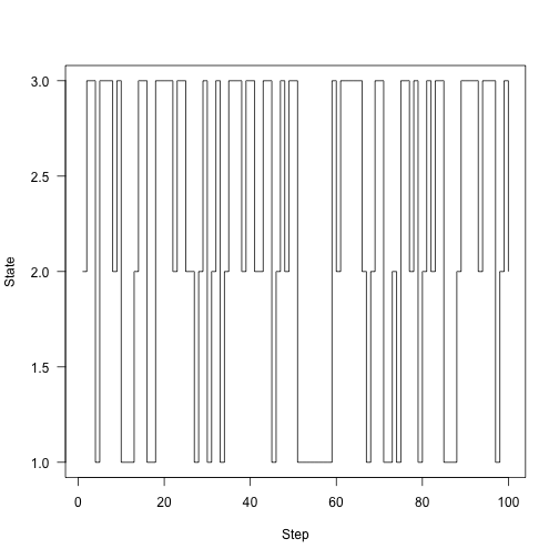
Rather than plotting state, plot the fraction of time that we were in each state over time:

1 2 3 4

plot(cummean(samples == 1), type="l", ylim=c(0, 1), xlab="Step", ylab="y", las=1) lines(cummean(samples == 2), col=2) lines(cummean(samples == 3), col=3)

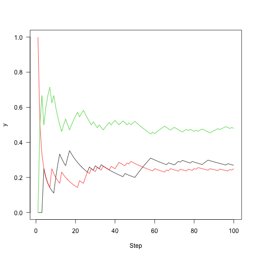
Run this out a little longer (5,000 steps)

1 2 3 4 5 6 7 8

n <- 5000 set.seed(1) samples <- run(1, P, n) plot(cummean(samples == 1), type="l", ylim=c(0, 1), log="x", xlab="Step", ylab="y", las=1) lines(cummean(samples == 2), col=2) lines(cummean(samples == 3), col=3) abline(h=v, lty=2, col=1:3)

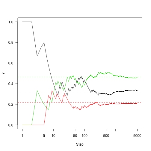
A sufficient (but not necessary) condition for the existance of a stationary distribution is Detailed Balance, which says:

This imples that the chain is reversible. The reason why this condition implies that a stationary distribution exists is that it implies

Summing both sides of the detailed balance equation over states $j$

The term on the left is equal to the $k$th element of $\vec\pi^*\mathbf{P}$ and the term on the right can be factored:

Then, because $\sum_j P(k \to j) = 1$ (because $P$ is a transition probability function, by the law of total probability things go somewhere with probability 1), so the right hand side is $\pi_k^*$, so we have

which holds for all $k$ so

So the key point here is: Markov chains are neat and well understood things, with some nice properties. Markov chains have stationary distributions, and if we run them for long enough we can just look at the where the chain is spending its time and get a reasonable estimate of that stationary distribution.

The Metropolis algorithm

This is the simplest MCMC algorithm. This section is not intended to show how to design efficient MCMC samplers, but just to see that they do in fact work. What we’re going to do is have some distribution that we want to sample from, and we’re going to be able to evaluate some function $f(x)$ that is proportional to the probability density of the target distribution (that is, if $p(x)$ is the probability density function itself, $f(x) \propto p(x)$, i.e., $f(x) = p(x) / Z$, where $Z = \int f(x) \mathrm{d} x$). Note that $x$ might be a vector or a scalar.

We also need a probability density function $P$ that we can draw samples from. For the simplest algorithm, this proposal distribution is symmetric, that is $P(x\to x^\prime) = P(x^\prime \to x)$.

The algorithm proceeds as follows.

1. Start in some state $x_t$.
2. Propose a new state $x^\prime$
3. Compute the “acceptance probability”
4. Draw some uniformly distributed random number $u$ from $[0,1]$; if $u < \alpha$ accept the point, setting $x{t+1} = x^\prime$. Otherwise reject it and set $x{t+1} = x_t$.

Note that in step 3 above, the unknown normalising constant drops out because

This will generate a series of samples ${x0, x1, \ldots}$. Note that where the proposed sample is rejected, the same value will be present in consecutive samples.

Note also that these are not independent samples from the target distribution; they are dependent samples; that is, sample $x_t$ depends on $x_{t-1}$ and so on. However, because the chain approaches a stationary distribution, this dependence will not matter so long as we sample enough points.

MCMC sampling in 1d (single parameter) problems

Here is a target distribution to sample from. It’s the weighted sum of two normal distributions. This sort of distribution is fairly straightforward to sample from, but let’s draw samples with MCMC. The probability density function is

This is a contrived example, but distributions like this are not totally impossible, and might arise when sampling things from a mixture (such as human heights, which are bimodal due to sexual dimorphism).

Fairly arbitrarily, here are some parameters and the definition of the target density.

1 2 3 4 5 6

p <- 0.4 mu <- c(-1, 2) sd <- c(.5, 2) f <- function(x) p * dnorm(x, mu[1], sd[1]) + (1-p) * dnorm(x, mu[2], sd[2])

Here is the probability density plotted over the “important” part of the domain (in general, this may not even be known!)

1	curve(f(x), col="red", -4, 8, n=301, las=1)

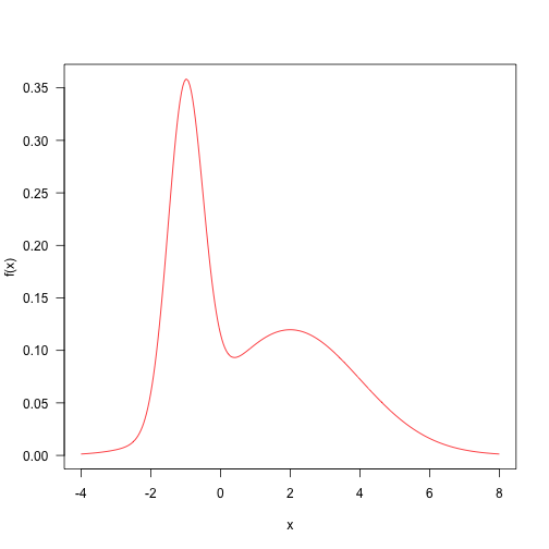
Let’s define a really simple minded proposal algorithm that samples from a normal distribution centred on the current point with a standard deviation of 4

1	q <- function(x) rnorm(1, x, 4)

This implements the core algorithm, as described above:

1 2 3 4 5 6 7 8 9 10 11

step <- function(x, f, q) { ## Pick new point xp <- q(x) ## Acceptance probability: alpha <- min(1, f(xp) / f(x)) ## Accept new point with probability alpha: if (runif(1) < alpha) x <- xp ## Returning the point: x }

And this just takes care of running the MCMC for a number of steps. It will start at point x return a matrix with nsteps rows and the same number of columns as x has elements. If run on scalar x it will return a vector.

1 2 3 4 5 6

run <- function(x, f, q, nsteps) { res <- matrix(NA, nsteps, length(x)) for (i in seq_len(nsteps)) res[i,] <- x <- step(x, f, q) drop(res) }

We pick a place to start (how about -10, just to pick a really poor point)

1	res <- run(-10, f, q, 1000)

Here are the first 1000 steps of the Markov chain, with the target density on the right:

1 2 3 4 5 6

layout(matrix(c(1, 2), 1, 2), widths=c(4, 1)) par(mar=c(4.1, .5, .5, .5), oma=c(0, 4.1, 0, 0)) plot(res, type="s", xpd=NA, ylab="Parameter", xlab="Sample", las=1) usr <- par("usr") xx <- seq(usr[3], usr[4], length=301) plot(f(xx), xx, type="l", yaxs="i", axes=FALSE, xlab="")

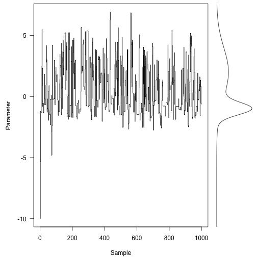
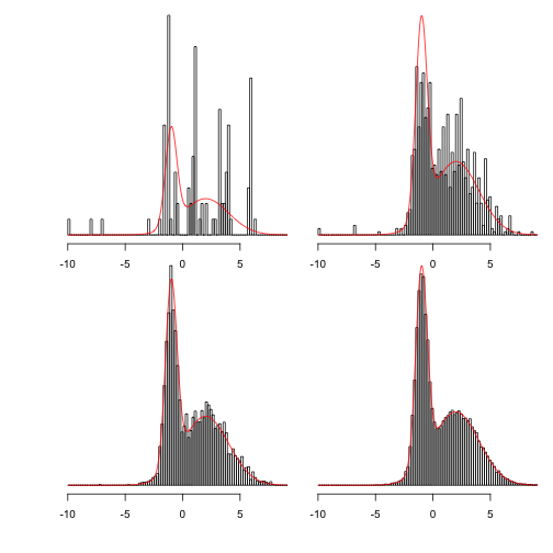
Even with only a thousand (non-independent) samples, we’re starting to resemble the target distribution fairly well.

1 2 3 4

hist(res, 50, freq=FALSE, main="", ylim=c(0, .4), las=1, xlab="x", ylab="Probability density") z <- integrate(f, -Inf, Inf)$value curve(f(x) / z, add=TRUE, col="red", n=200)

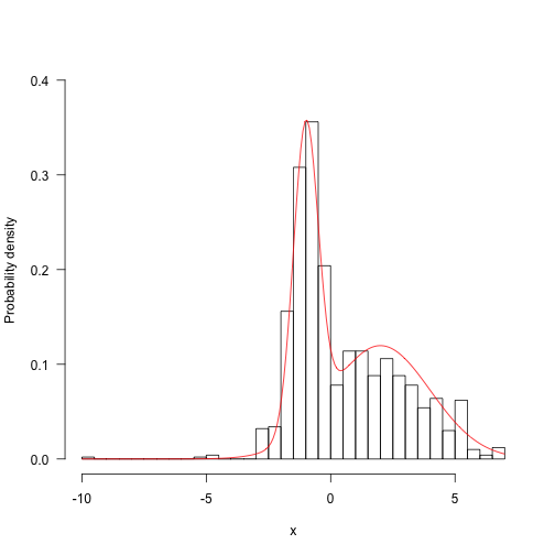
Run for longer and things start looking a bunch better:

1 2 3 4 5 6

set.seed(1) res.long <- run(-10, f, q, 50000) hist(res.long, 100, freq=FALSE, main="", ylim=c(0, .4), las=1, xlab="x", ylab="Probability density", col="grey") z <- integrate(f, -Inf, Inf)$value curve(f(x) / z, add=TRUE, col="red", n=200)

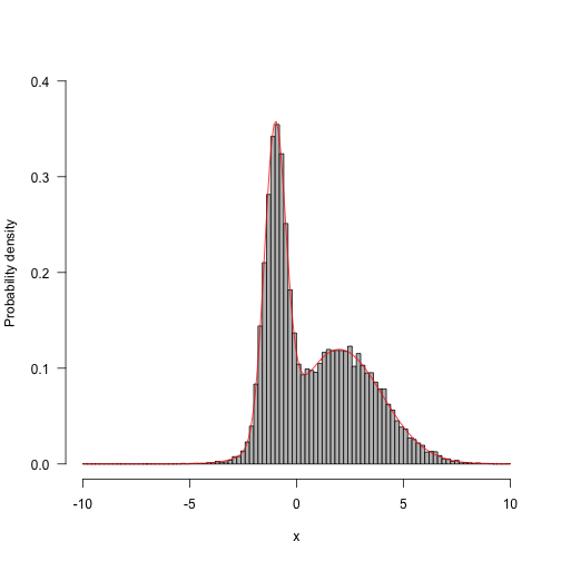
Now, run with different proposal mechanisms - one with a very wide standard deviation (33 units) and the other with a very small standard deviation (3 units).

1 2	res.fast <- run(-10, f, function(x) rnorm(1, x, 33), 1000) res.slow <- run(-10, f, function(x) rnorm(1, x, .3), 1000)

Here is the same plot as above – note the different ways that the three traces are moving around.

1 2 3 4 5 6 7

layout(matrix(c(1, 2), 1, 2), widths=c(4, 1)) par(mar=c(4.1, .5, .5, .5), oma=c(0, 4.1, 0, 0)) plot(res, type="s", xpd=NA, ylab="Parameter", xlab="Sample", las=1, col="grey") lines(res.fast, col="red") lines(res.slow, col="blue") plot(f(xx), xx, type="l", yaxs="i", axes=FALSE)

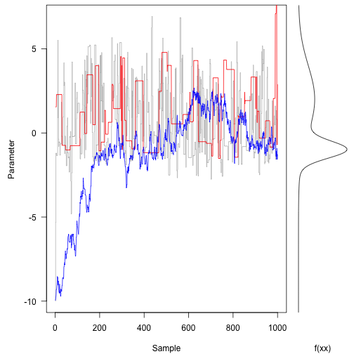
The original (grey line) trace is bouncing around quite freely.

In contrast, the red trace (large proposal moves) is suggesting terrible spaces in probability space and rejecting most of them. This means it tends to stay put for along time at once space.

The blue trace proposes small moves that tend to be accepted, but it moves following a random walk for most of the trajectory. It takes hundreds of iterations to even reach the bulk of the probability density.

You can see the effect of different proposal steps in the autocorrelation among subsequent parameters – these plots show the decay in autocorrelation coefficient between steps of different lags, with the blue lines indicating statistical independence.

1 2 3 4

par(mfrow=c(1, 3), mar=c(4, 2, 3.5, .5)) acf(res.slow, las=1, main="Small steps") acf(res, las=1, main="Intermediate") acf(res.fast, las=1, main="Large steps")

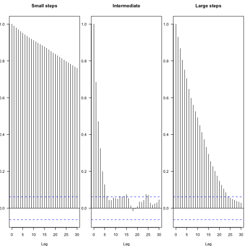
From this, one can calculate the effective number of independent samples:

1	coda::effectiveSize(res)

1 2	## var1 ## 187

1	coda::effectiveSize(res.fast)

1 2	## var1 ## 33.19

1	coda::effectiveSize(res.slow)

1 2	## var1 ## 5.378

The chains both “mix” worse than that first one.

This shows more clearly what happens as the chains are run for longer:

1 2 3 4 5 6 7

n <- 10^(2:5) samples <- lapply(n, function(n) run(-10, f, q, n)) xlim <- range(sapply(samples, range)) br <- seq(xlim[1], xlim[2], length=100) hh <- lapply(samples, function(x) hist(x, br, plot=FALSE)) ylim <- c(0, max(f(xx)))

Showing 100, 1,000, 10,000 and 100,000 steps:

1 2 3 4 5 6

par(mfrow=c(2,2), mar=rep(.5, 4), oma=c(4, 4, 0, 0)) for (h in hh) { plot(h, main="", freq=FALSE, yaxt="n", ylim=range(h$density, ylim)) curve(f(x), add=TRUE, col="red", n=300) }

MCMC In two dimensions

This is a function that makes a multivariate normal density given a vector of means (centre of the distribution) and variance-covariance matrix.

1 2 3 4 5 6 7 8 9 10

make.mvn <- function(mean, vcv) { logdet <- as.numeric(determinant(vcv, TRUE)$modulus) tmp <- length(mean) * log(2 * pi) + logdet vcv.i <- solve(vcv) function(x) { dx <- x - mean exp(-(tmp + rowSums((dx %*% vcv.i) * dx))/2) } }

As above, define the target density to be the sum of two mvns (this time unweighted):

1 2 3 4 5 6 7 8 9 10 11 12 13 14 15 16

mu1 <- c(-1, 1) mu2 <- c(2, -2) vcv1 <- matrix(c(1, .25, .25, 1.5), 2, 2) vcv2 <- matrix(c(2, -.5, -.5, 2), 2, 2) f1 <- make.mvn(mu1, vcv1) f2 <- make.mvn(mu2, vcv2) f <- function(x) f1(x) + f2(x) x <- seq(-5, 6, length=71) y <- seq(-7, 6, length=61) xy <- expand.grid(x=x, y=y) z <- matrix(apply(as.matrix(xy), 1, f), length(x), length(y)) image(x, y, z, las=1) contour(x, y, z, add=TRUE)

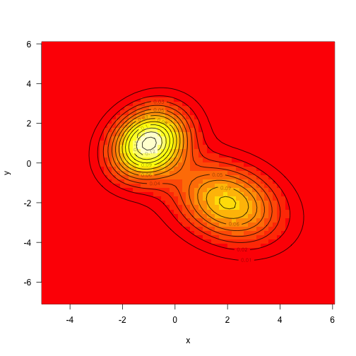
Sampling from multivariate normals is also fairly straightforward, but we’ll draw samples from this using MCMC.

There are a bunch of different strategies here – we could propose moves in both dimensions simultaneously, or we could sample along each axis independently. Both strategies will work, though they will again differ in how rapidly they mix.

Assume that we don’t actually know how to sample from a mvn (it’s not actually hard, but this is simpler), let’s make a proposal distribution that is uniform in two dimensions, sampling from the square with width ‘d’ on each side.

1 2 3 4 5 6 7 8 9 10

q <- function(x, d=8) x + runif(length(x), -d/2, d/2) x0 <- c(-4, -4) set.seed(1) samples <- run(x0, f, q, 1000) image(x, y, z, xlim=range(x, samples[,1]), ylim=range(x, samples[,2])) contour(x, y, z, add=TRUE) lines(samples[,1], samples[,2], col="#00000088")

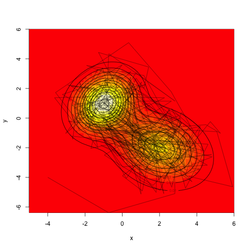
Drawing a ton of samples”

1 2	set.seed(1) samples <- run(x0, f, q, 100000)

Compare the sampled distribution against the known distribution:

1 2	smoothScatter(samples) contour(x, y, z, add=TRUE)

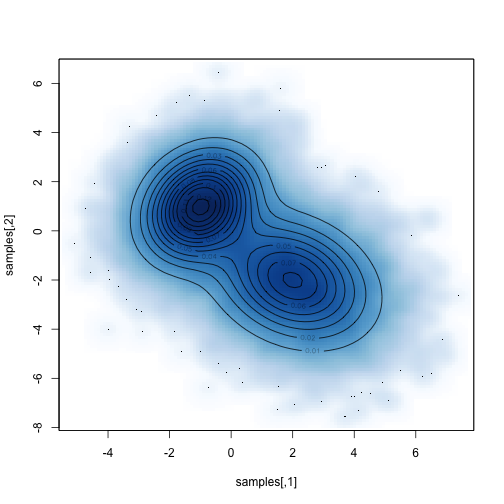
Then we can easily do things with the samples that are difficult to do directly. For example, what is themarginal distribution of parameter 1:

1 2	hist(samples[,1], freq=FALSE, main="", xlab="x", ylab="Probability density")

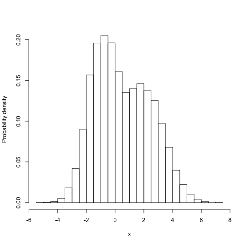
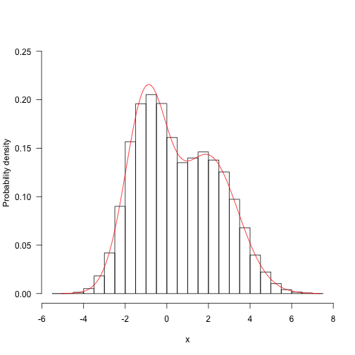
(this is the distribution that the first paramter takes, averaged over all the possible values that the second parameter might take, weighted by their probability).

Computing this properly is tricky - we need to integrate over all possible values of the second parameter for each value of the first. Then, because the target function is not itself normalised, we have to divide that through by the value of integrating over the first dimension (this is the total area under the distribution).

1 2 3 4 5 6 7 8 9 10 11 12

m <- function(x1) { g <- Vectorize(function(x2) f(c(x1, x2))) integrate(g, -Inf, Inf)$value } xx <- seq(min(samples[,1]), max(samples[,1]), length=201) yy <- sapply(xx, m) z <- integrate(splinefun(xx, yy), min(xx), max(xx))$value hist(samples[,1], freq=FALSE, main="", las=1, xlab="x", ylab="Probability density", ylim=c(0, 0.25)) lines(xx, yy/z, col="red")

Comments

 

Recent Posts

• Figure functions
• Modifying data with lookup tables
• Organizing the project directory
• How long is a function?
• Excel and line endings

Copyright © 2016 - Rich FitzJohn & Daniel Falster - Powered by Octopress