Analyzing The Papers Behind Facebook's Computer Vision Approach
Analyzing The Papers Behind Facebook's Computer Vision Approach
Introduction
You know that company called Facebook? Yeah, the one that has 1.6 billion people hooked on their website. Take all of the happy birthday posts, embarrassing pictures of you as a little kid, that one family relative that likes every single one of your statuses, and you have a whole lot of data to analyze.
In terms of analyzing the images, Facebook has undoubtedly made great progress with deep CNNs. A little over a week ago, the team at Facebook AI Research (FAIR) published a blog post detailing the computer vision techniques that are behind some of their object segmentation algorithms. In this post, we’ll go into summarizing and explaining the 3 papers that the blog referenced.

The main pipeline that FAIR utilizes goes as follows. Images are fed into a DeepMask segmentation framework. The segments are refined through a SharpMask model and classified with MultiPathNet. Let’s look at how each of these components operates separately.
DeepMask
Introduction
Written by Pedro Pinheiro, Roman Collobert, and Piotr Dollar, this paper is titled “Learning to Segment Object Candidates”. The authors approach the task of object segmentation through a model that, given an image patch, first outputs a segmentation mask and then outputs the probability that the patch is centered on a full object. That process is applied over the whole image so that a mask can be created for each object. This whole process is done through just one CNN, as both components share many of the layers in the network.
Inputs and Outputs
Let’s first visualize what want this model to do. Given an input image, we want the network to output a set of masks, or outlines, for each object. We can think of each input image as containing a set of patches (crops of the original image). For each input patch, the output is a binary mask that outlines the shape of the main object as well as a score (between -1 and 1) for how likely the input patch is to contain an object.
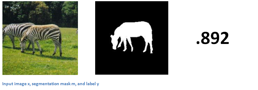
Each training example will need to contain these 3 elements (Side Note: Examples with a 1 label need to contain an object that is roughly centered, fully contained in the image, and in a given scale range). The model applies this process at multiple scales and locations on the image (this is the patch set that we were talking about earlier). The results are then aggregated together to form one final image with all of the masks. Now, let’s take a look at the how this model is structured.
Network Architecture
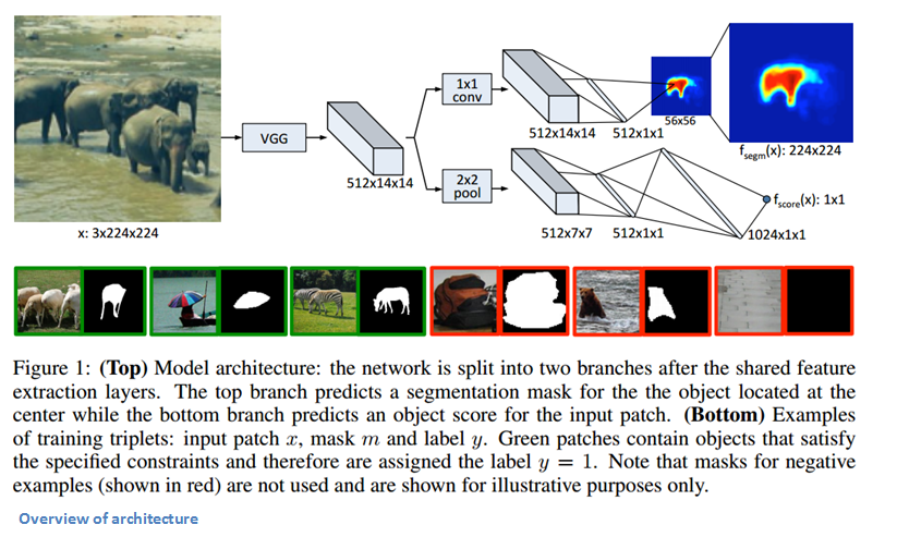
The network was pre-trained for classification on ImageNet (Transfer Learning works. Use it). The image is fed through a VGG-like model (without the fully connected layers) with eight 3x3 conv layers and five 2x2 maxpool layers. Depending on your input image dimensions, you will get a certain output volume (in this case, 512x14x14).
Input: 3 x h x w
Output: 512 x h/16 x w/16
Then, the model separates into the 2 components described earlier. One head tackles segmentation while the other determines whether or not there is an object in the image.
Segmentation Head
Now we take our output volume, pass it through a network-in-network layer and a ReLU layer. Then, we have a layer ofw’ x h’ (where w’ and h’ are less than the h and w of the original image) pixel classifiers which determine whether or not a given pixel is part of the object in the center of the image (If you have a 28x28 sized original image, there will be less than 784 classifiers). We then look at the outputs of these classifiers, bilinearly upsample the output to fit the full original resolution, and obtain a black and white binary mask (1’s for yes classification and zeros for no classification).
Objectness Head
The other component of the network determines if the image contains an object that is centered and at an appropriate scale. Putting the output of VGG-like layers through a 2x2 maxpool, a dropout unit, and two fully connected layers, we’re able to obtain our “objectness” score.
Training
Both components of the network are trained simultaneously as the loss function is a sum of logistic regression losses (one for the objectness head and one for every location in the segmentation head). Backpropagation alternates between going through the segmentation head and the objectness head. Data augmentation techniques were used to improve the model. The model was trained with stochastic gradient descent on an Nvidia Tesla K40m GPU for around 5 days.
Why This Paper is Cool
A single convolutional neural network. We didn’t need an extra object proposal step or some complex training pipeline. There is a certain simplicity to this model which helps the network’s flexibility as well as its efficiency and speed.
SharpMask
Introduction
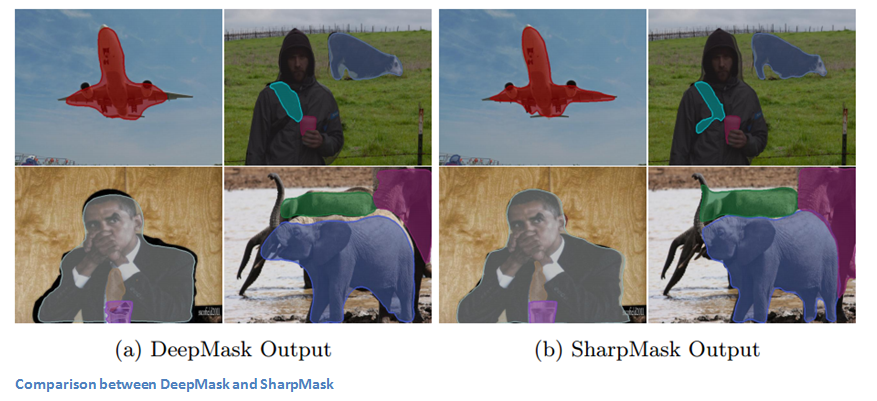
The previous group (along with Tsung-Yi Lin) also authored the paper titled “Learning to Refine Object Segments”. Evidenced by the title, the paper aims to refine the segmentation masks created in the DeepMask model. The main issue with DeepMask is that it uses a simple feed forward network that is successful in creating “coarse object masks”, but not in “pixel-accurate segmentations”. The reason for this is that, as you may remember, there is a bilinear up sampling that takes place in order to fit the full size of the image. This causes rough and imprecise alignment with the object boundaries. To address this, the SharpMask model works to combine information from the low-level features that comes from the early layers with the high-level object information that comes from the layers deeper in the network. The model does this by first creating a rough mask for each input patch (DeepMask’s job), and then passing it through different refinement modules throughout the network. Let’s look at the specifics.
Network Architecture
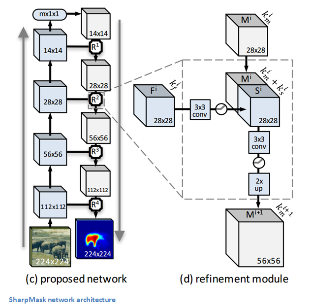
The motivation behind SharpMask’s architecture is that because object-level (high-level) information is needed to find a precise segmentation mask, we need to use a top-down approach that first creates a coarse outline but then integrates important low-level information from earlier layers. As you can see from the above picture, the original input first goes through the DeepMask pipeline to obtain a rough segmentation. It then is exposed to a series of refinement modules that allow for a more precise upsampling back to the original dimensions of the image.
Refinement Module
Let’s dig a little deeper into the specifics of this refinement module. The goal of this module is to counter the effects of the pooling layers in the DeepMask pipeline (the layers that shrunk the 224x224 image to 14x14) by upsampling the generated masks in a way that also takes into account the feature maps that were created in the bottom-up pass (You can think of DeepMask = bottom-up and Refinement Module = top-down). A mathematical way of looking at it is that the refinement module R is a function that generates an upsampled mask M that is a function of the mask in the previous layer as well as a function of the feature map F. The number of refinement modules used would be equal to the number of pooling layers used in the DeepMask pipeline.

Now, what exactly goes on in that function R? Glad you asked. A naïve approach would be to just concatenate M and F since they have the same width and height. The problem there lies in the depth channels of each of those components. The number of depth channels for feature maps can be much larger compared to that of the mask. Therefore, concatenating would put too much of an emphasis on F. The solution would be to simply reduce the number of depth channels for F by applying a 3x3 conv layer, then concatenating M, going through another 3x3 conv, and finally using a bilinear upsampling (see network architecture image to follow along).
Training
The same training data that DeepMask uses also applies for SharpMask. We need input patches with binary masks as well as labels. The DeepMask layers are trained first. The weights are then frozen as the refinement modules begin their training.
Why This Paper is Cool
This paper was able to build on DeepMask’s approach while introducing a new and easy-to-use module. The authors creatively realized that they could obtain more precise segmentations by just integrating the low level information that was available in the early layers of the DeepMask pipeline.
MultiPathNet
Introduction
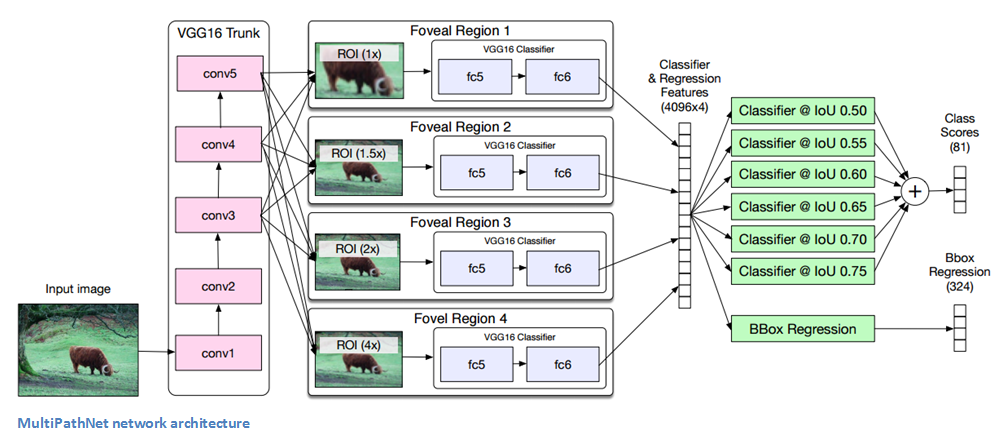
DeepMask generates coarse segmentation masks. SharpMask refines those outlines. MultiPathNet has the job of identifying or classifying the objects in the masks. A group consisting of Sergey Zagoruyko, Adam Lerer, Tsung-Yi Lin, Pedro Pinheiro, Sam Gross, Soumith Chintala, and Piotr Dollar published the paper titled “A MultiPath Network for Object Detection”. The goal of this paper is to improve on object detection techniques by focusing on higher precision localization as well as difficult images with scale variance, heavy occlusion, and clutter. This model takes Fast R-CNN as a starting point, so if you haven’t already, check out that paper or look at my previous blog post for a summary. Basically, this model is a way of implementing Fast R-CNN with DeepMask/SharpMask object proposals. The 3 main modifications that this paper introduced include skip connections, foveal regions, and an integral loss function. Let’s look at the network architecture before diving into each of those.
Network Architecture/Foveal Regions
As with Fast R-CNN, we pass the input image through a VGG network without the fully connected layers. ROI pooling is used to extract features of the region proposals (If we remember from the Fast R-CNN paper, ROI pooling is a way of mapping features of the image to a feature map of fixed spatial extent that describes the regions). For each object proposal, we then create 4 different region crops for the purpose of viewing the object at multiple scales. These are the “foveal regions” discussed in the intro. These region crops are fed through fully connected layers, the outputs are concatenated, and the network splits into a classification and a regression head. The authors hypothesize that these foveal regions help with localization precision because the network is able to view the image at different scales and with different context around the object of interest.
Skip Connections
Due to Fast R-CNN’s architecture, an input image of 32x32 will quickly get reduced to 2x2 after the last VGG conv layer. ROI pooling will create a 7x7 map, but we’ve still lost a lot of the original spatial information. To combat this, we concatenate the features from the conv3, conv4, and conv5 layers and then feed that into the foveal classifier. The paper states that this concatenation “gives the classifier access to information from features at multiple locations”.
Integral Loss
Don’t want to go too much into this one since I feel like the math will undoubtedly be much better explained in the paper itself, but the general idea is the authors came up with a loss function that performs better while testing with multiple intersection over union (IoU) values.
Why This Paper is Cool
If you like Fast R-CNN, I think you’ll definitely like this model. It takes the main ideas of using VGG Net and ROI pooling, while also introducing a way to obtain more precise localizations and classifications through foveal regions, skip connections, and integral loss.
Facebook kinda has this CNN stuff down.
If anyone has anything to add or different explanations of any of the papers, let me know in the comments!
The code for DeepMask and SharpMask. The code for MultiPathNet.
Dueces.
Sources


 浙公网安备 33010602011771号