(转)How Transformers Work --- The Neural Network used by Open AI and DeepMind
How Transformers Work
--- The Neural Network used by Open AI and DeepMind
Original English Version link:https://towardsdatascience.com/transformers-141e32e69591
Chinese version by 量子位。
本文的主要内容:RNN, LSTM, Attention, CNN, Transformer, Self-Attention, Multi-head Attention 等常见的用于 language 或者 时序编码的网络与相关技术概览。
Overview
I give an overview of how Transformers work and why this is the technique used for sequence transduction. If you want to understand in depth how the model works and all its nuances, I recommend the following posts, articles and videos that I used as a base for summarizing the technique
- The Unreasonable Effectiveness of Recurrent Neural Networks
- Understanding LSTM Networks
- Visualizing A Neural Machine Translation Model
- The Illustrated Transformer
- The Transformer — Attention is all you need
- The Annotated Transformer
- Attention is all you need attentional neural network models
- Self-Attention For Generative Models
- OpenAI GPT-2: Understanding Language Generation through Visualization
- WaveNet: A Generative Model for Raw Audio
Transformers are a type of neural network architecture that have been gaining popularity. Transformers were recently used by OpenAI in their language models, and also used recently by DeepMind for AlphaStar — their program to defeat a top professional Starcraft player.
Transformers were developed to solve the problem of sequence transduction, or neural machine translation. That means any task that transforms an input sequence to an output sequence. This includes speech recognition, text-to-speech transformation, etc..

Sequence transduction. The input is represented in green, the model is represented in blue, and the output is represented in purple. GIF taken from 3
For models to perform sequence transduction, it is necessary to have some sort of memory. For example let’s say that we are translating the following sentence to another language (French):
“The Transformers” are a Japanese [[hardcore punk]] band. The band was formed in 1968, during the height of Japanese music history”
In this example, the word “the band” in the second sentence refers to the band “The Transformers” introduced in the first sentence. When you read about the band in the second sentence, you know that it is referencing to the “The Transformers” band. That may be important for translation. There are many examples, where words in some sentences refer to words in previous sentences.
For translating sentences like that, a model needs to figure out these sort of dependencies and connections. Recurrent Neural Networks (RNNs) and Convolutional Neural Networks (CNNs) have been used to deal with this problem because of their properties. Let’s go over these two architectures and their drawbacks.
Recurrent Neural Networks
Recurrent Neural Networks have loops in them, allowing information to persist.
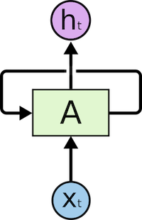
The input is represented as x_t
In the figure above, we see part of the neural network, A, processing some input x_t and outputs h_t. A loop allows information to be passed from one step to the next.
The loops can be thought in a different way. A Recurrent Neural Network can be thought of as multiple copies of the same network, A, each network passing a message to a successor. Consider what happens if we unroll the loop:

An unrolled recurrent neural network
This chain-like nature shows that recurrent neural networks are clearly related to sequences and lists. In that way, if we want to translate some text, we can set each input as the word in that text. The Recurrent Neural Network passes the information of the previous words to the next network that can use and process that information.
The following picture shows how usually a sequence to sequence model works using Recurrent Neural Networks. Each word is processed separately, and the resulting sentence is generated by passing a hidden state to the decoding stage that, then, generates the output.
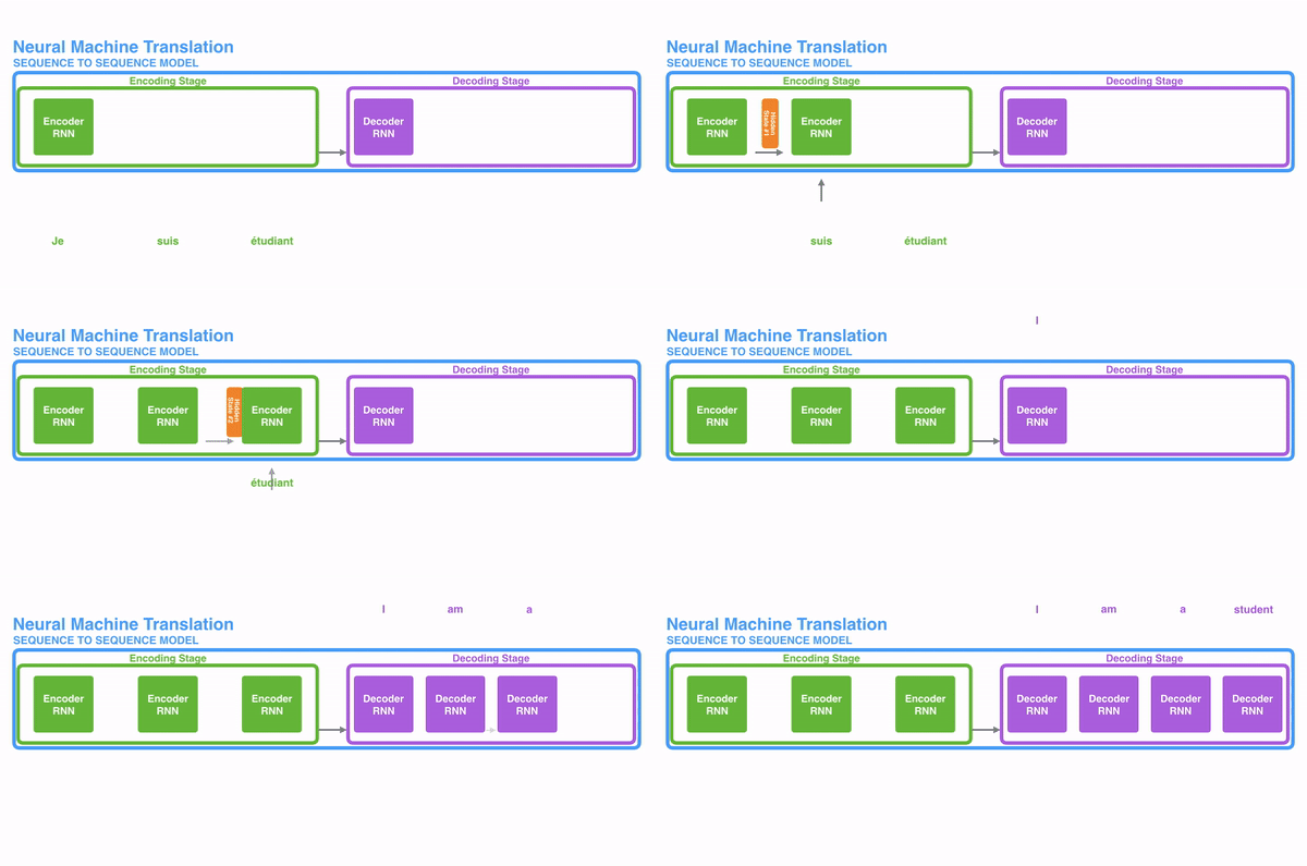
GIF taken from 3
The problem of long-term dependencies
Consider a language model that is trying to predict the next word based on the previous ones. If we are trying to predict the next word of the sentence “the clouds in the sky”, we don’t need further context. It’s pretty obvious that the next word is going to be sky.
In this case where the difference between the relevant information and the place that is needed is small, RNNs can learn to use past information and figure out what is the next word for this sentence.
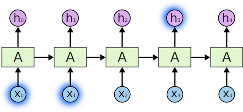
Image taken from 6
But there are cases where we need more context. For example, let’s say that you are trying to predict the last word of the text: “I grew up in France… I speak fluent …”. Recent information suggests that the next word is probably a language, but if we want to narrow down which language, we need context of France, that is further back in the text.
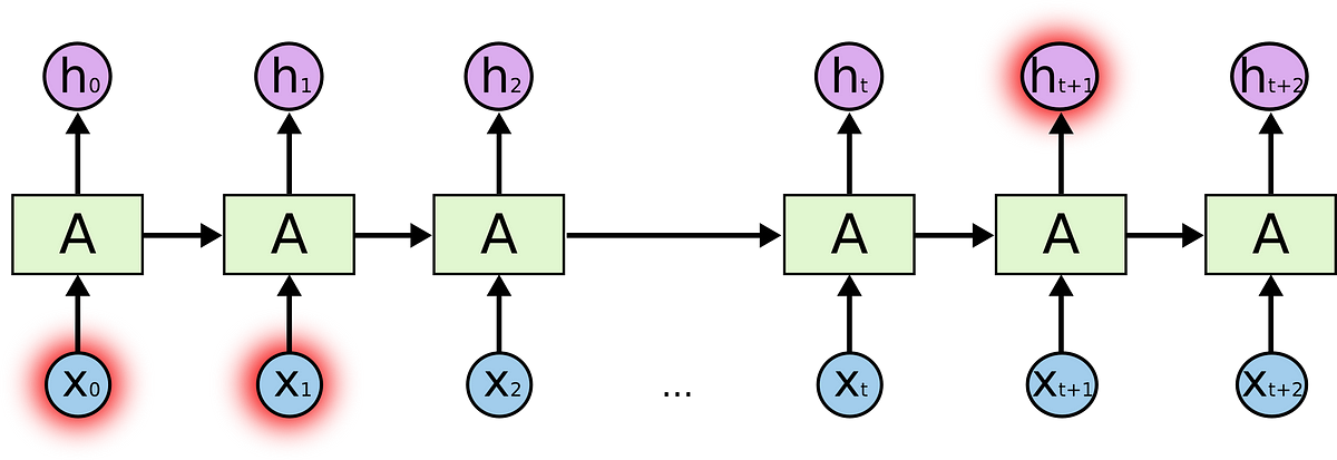
Image taken from 6
RNNs become very ineffective when the gap between the relevant information and the point where it is needed become very large. That is due to the fact that the information is passed at each step and the longer the chain is, the more probable the information is lost along the chain.
In theory, RNNs could learn this long-term dependencies. In practice, they don’t seem to learn them. LSTM, a special type of RNN, tries to solve this kind of problem.
information is lost along the chain.
In theory, RNNs could learn this long-term dependencies. In practice, they don’t seem to learn them. LSTM, a special type of RNN, tries to solve this kind of problem.
Long-Short Term Memory (LSTM)
When arranging one’s calendar for the day, we prioritize our appointments. If there is anything important, we can cancel some of the meetings and accommodate what is important.
RNNs don’t do that. Whenever it adds new information, it transforms existing information completely by applying a function. The entire information is modified, and there is no consideration of what is important and what is not.
LSTMs make small modifications to the information by multiplications and additions. With LSTMs, the information flows through a mechanism known as cell states. In this way, LSTMs can selectively remember or forget things that are important and not so important.
Internally, a LSTM looks like the following:
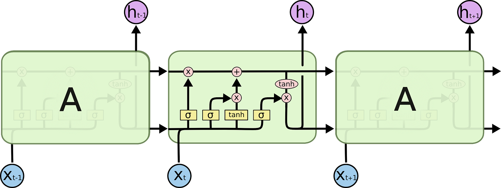
Image taken from 6
Each cell takes as inputs x_t (a word in the case of a sentence to sentence translation), the previous cell state and the output of the previous cell. It manipulates these inputs and based on them, it generates a new cell state, and an output. I won’t go into detail on the mechanics of each cell. If you want to understand how each cell works, I recommend Christopher’s blog post:
The problem with LSTMs
The same problem that happens to RNNs generally, happen with LSTMs, i.e. when sentences are too long LSTMs still don’t do too well. The reason for that is that the probability of keeping the context from a word that is far away from the current word being processed decreases exponentially with the distance from it.
That means that when sentences are long, the model often forgets the content of distant positions in the sequence. Another problem with RNNs, and LSTMs, is that it’s hard to parallelize the work for processing sentences, since you are have to process word by word. Not only that but there is no model of long and short range dependencies. To summarize, LSTMs and RNNs present 3 problems:
- Sequential computation inhibits parallelization
- No explicit modeling of long and short range dependencies
- “Distance” between positions is linear
Attention
To solve some of these problems, researchers created a technique for paying attention to specific words.
When translating a sentence, I pay special attention to the word I’m presently translating. When I’m transcribing an audio recording, I listen carefully to the segment I’m actively writing down. And if you ask me to describe the room I’m sitting in, I’ll glance around at the objects I’m describing as I do so.
Neural networks can achieve this same behavior using attention, focusing on part of a subset of the information they are given. For example, an RNN can attend over the output of another RNN. At every time step, it focuses on different positions in the other RNN.
To solve these problems, Attention is a technique that is used in a neural network. For RNNs, instead of only encoding the whole sentence in a hidden state, each word has a corresponding hidden state that is passed all the way to the decoding stage. Then, the hidden states are used at each step of the RNN to decode. The following gif shows how that happens.
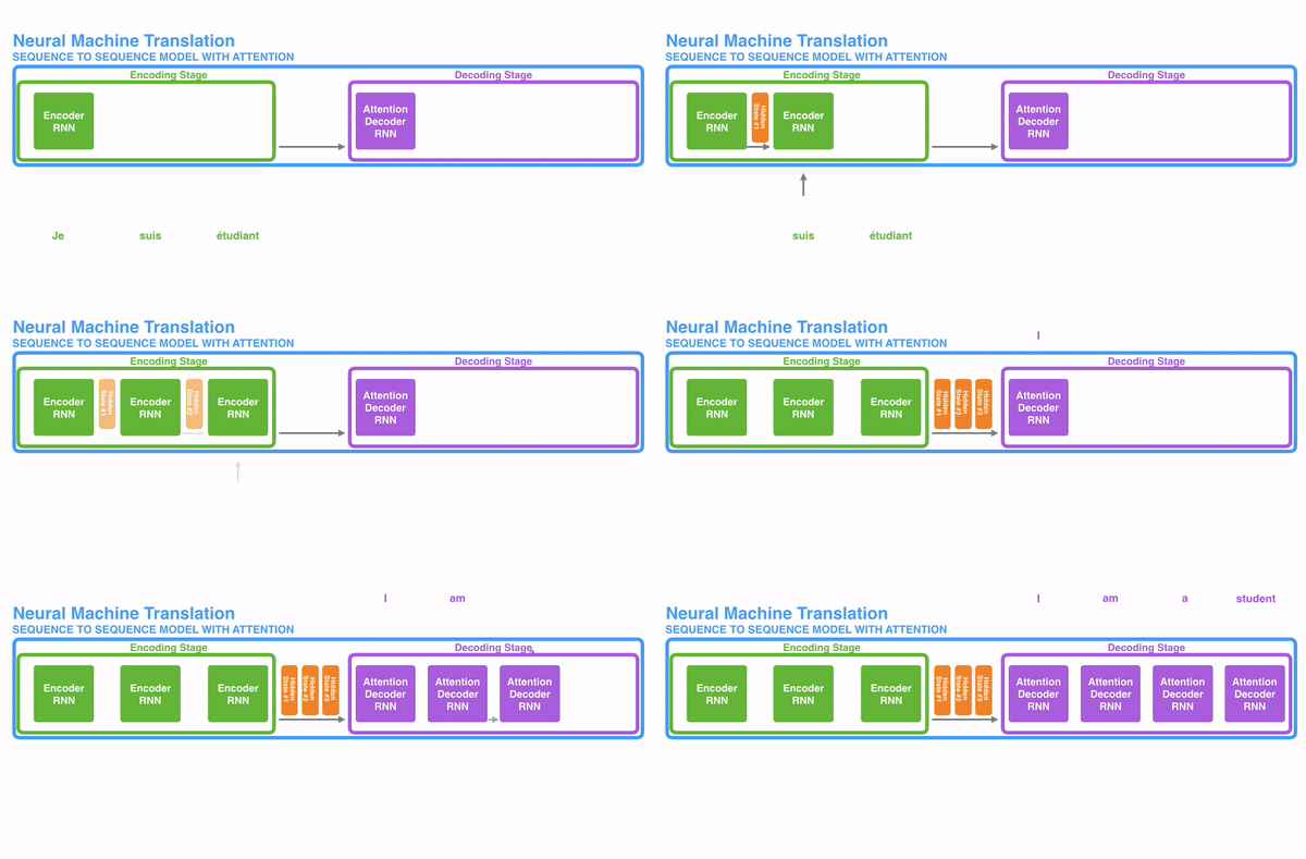
The green step is called the encoding stage and the purple step is the decoding stage. GIF taken from 3
The idea behind it is that there might be relevant information in every word in a sentence. So in order for the decoding to be precise, it needs to take into account every word of the input, using attention.
For attention to be brought to RNNs in sequence transduction, we divide the encoding and decoding into 2 main steps. One step is represented in greenand the other in purple. The green step is called the encoding stage and the purple step is the decoding stage.
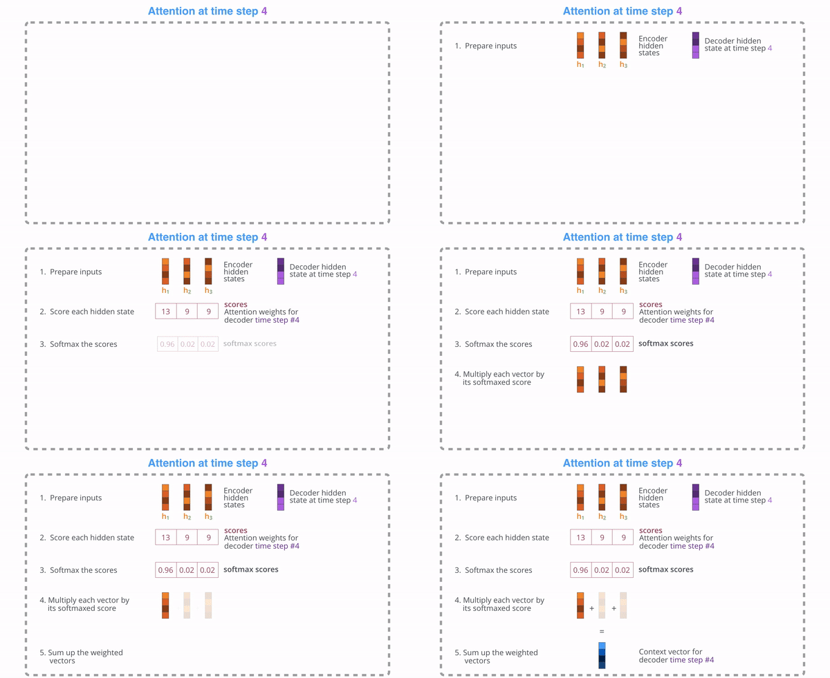
GIF taken from 3
The step in green in charge of creating the hidden states from the input. Instead of passing only one hidden state to the decoders as we did before using attention, we pass all the hidden states generated by every “word” of the sentence to the decoding stage. Each hidden state is used in the decoding stage, to figure out where the network should pay attention to.
For example, when translating the sentence “Je suis étudiant” to English, requires that the decoding step looks at different words when translating it.
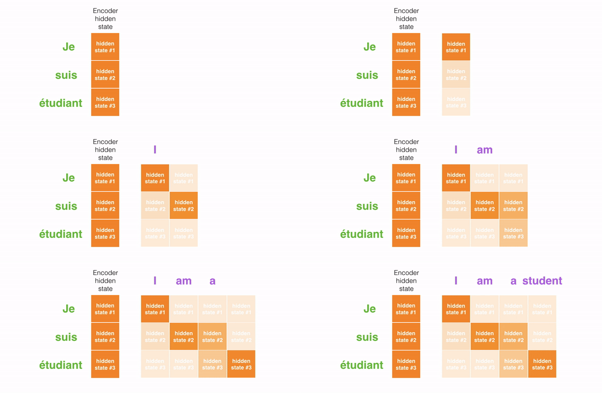
This gif shows how the weight that is given to each hidden state when translating the sentence “Je suis étudiant” to English. The darker the color is, the more weight is associated to each word. GIF taken from 3
Or for example, when you translate the sentence “L’accord sur la zone économique européenne a été signé en août 1992.” from French to English, and how much attention it is paid to each input.
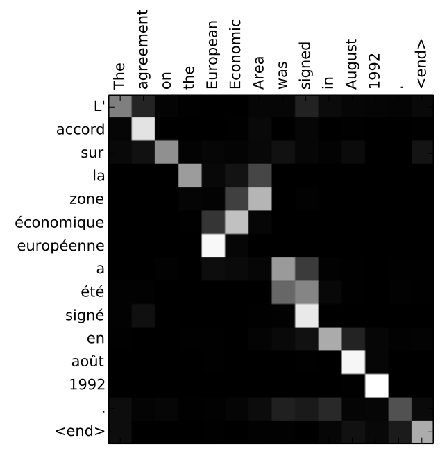
Translating the sentence “L’accord sur la zone économique européenne a été signé en août 1992.” to English. Image taken from 3
But some of the problems that we discussed, still are not solved with RNNs using attention. For example, processing inputs (words) in parallel is not possible. For a large corpus of text, this increases the time spent translating the text.
Convolutional Neural Networks
Convolutional Neural Networks help solve these problems. With them we can
- Trivial to parallelize (per layer)
- Exploits local dependencies
- Distance between positions is logarithmic
Some of the most popular neural networks for sequence transduction, Wavenet and Bytenet, are Convolutional Neural Networks.
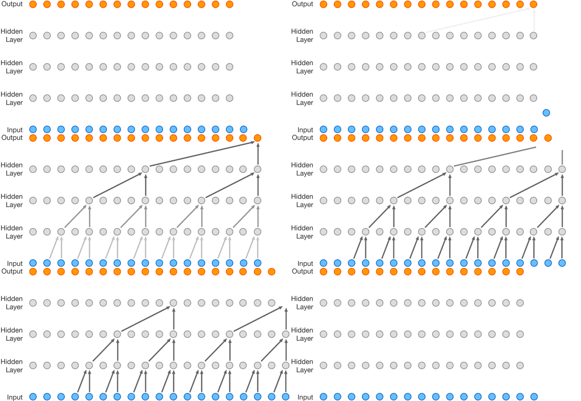
Wavenet, model is a Convolutional Neural Network (CNN). Image taken from 10
The reason why Convolutional Neural Networks can work in parallel, is that each word on the input can be processed at the same time and does not necessarily depend on the previous words to be translated. Not only that, but the “distance” between the output word and any input for a CNN is in the order of log(N) — that is the size of the height of the tree generated from the output to the input (you can see it on the GIF above. That is much better than the distance of the output of a RNN and an input, which is on the order of N.
The problem is that Convolutional Neural Networks do not necessarily help with the problem of figuring out the problem of dependencies when translating sentences. That’s why Transformers were created, they are a combination of both CNNs with attention.
Transformers
To solve the problem of parallelization, Transformers try to solve the problem by using Convolutional Neural Networks together with attention models.Attention boosts the speed of how fast the model can translate from one sequence to another.
Let’s take a look at how Transformer works. Transformer is a model that uses attention to boost the speed. More specifically, it uses self-attention.

The Transformer. Image taken from 4
Internally, the Transformer has a similar kind of architecture as the previous models above. But the Transformer consists of six encoders and six decoders.
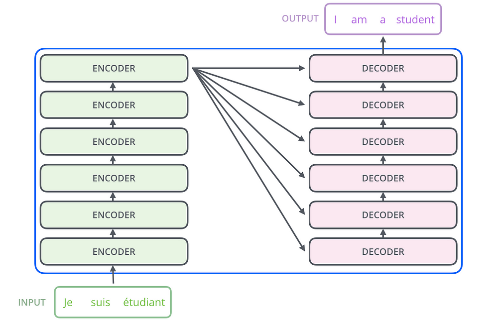
Image taken from 4
Each encoder is very similar to each other. All encoders have the same architecture. Decoders share the same property, i.e. they are also very similar to each other. Each encoder consists of two layers: Self-attention and a feed Forward Neural Network.
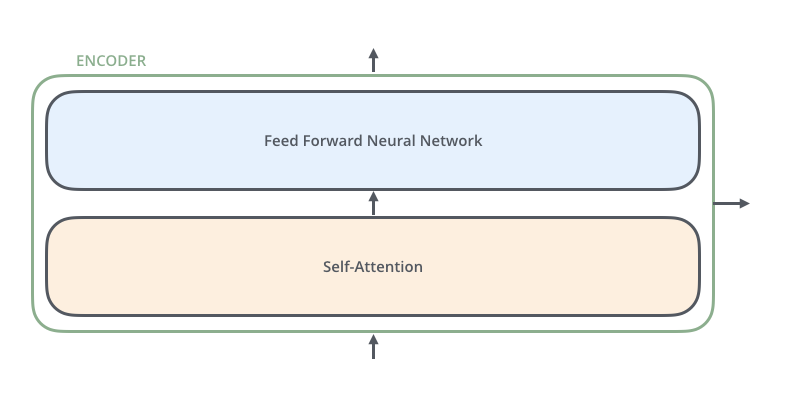
Image taken from 4
The encoder’s inputs first flow through a self-attention layer. It helps the encoder look at other words in the input sentence as it encodes a specific word. The decoder has both those layers, but between them is an attention layer that helps the decoder focus on relevant parts of the input sentence.
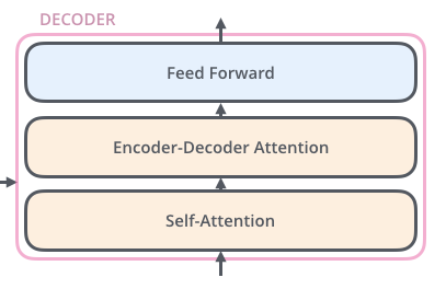
Image taken from 4
Self-Attention
Note: This section comes from Jay Allamar blog post
Let’s start to look at the various vectors/tensors and how they flow between these components to turn the input of a trained model into an output. As is the case in NLP applications in general, we begin by turning each input word into a vector using an embedding algorithm.

Each word is embedded into a vector of size 512. We’ll represent those vectors with these simple boxes.
The embedding only happens in the bottom-most encoder. The abstraction that is common to all the encoders is that they receive a list of vectors each of the size 512.
In the bottom encoder that would be the word embeddings, but in other encoders, it would be the output of the encoder that’s directly below. After embedding the words in our input sequence, each of them flows through each of the two layers of the encoder.
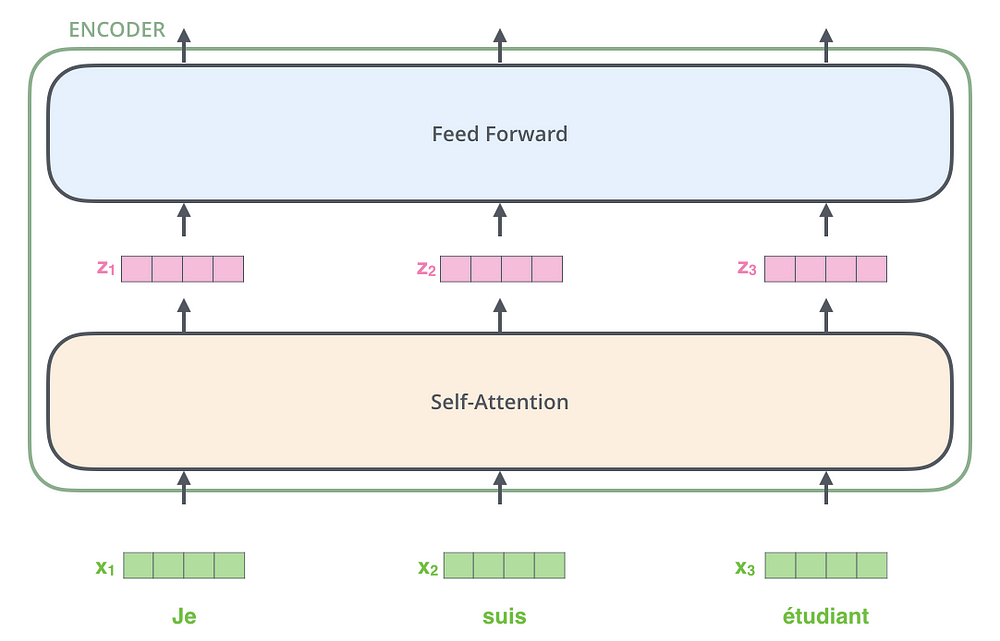
Here we begin to see one key property of the Transformer, which is that the word in each position flows through its own path in the encoder. There are dependencies between these paths in the self-attention layer. The feed-forward layer does not have those dependencies, however, and thus the various paths can be executed in parallel while flowing through the feed-forward layer.
Next, we’ll switch up the example to a shorter sentence and we’ll look at what happens in each sub-layer of the encoder.
Self-Attention
Let’s first look at how to calculate self-attention using vectors, then proceed to look at how it’s actually implemented — using matrices.
The first step in calculating self-attention is to create three vectors from each of the encoder’s input vectors (in this case, the embedding of each word). So for each word, we create a Query vector, a Key vector, and a Value vector. These vectors are created by multiplying the embedding by three matrices that we trained during the training process.
Notice that these new vectors are smaller in dimension than the embedding vector. Their dimensionality is 64, while the embedding and encoder input/output vectors have dimensionality of 512. They don’t HAVE to be smaller, this is an architecture choice to make the computation of multiheaded attention (mostly) constant.
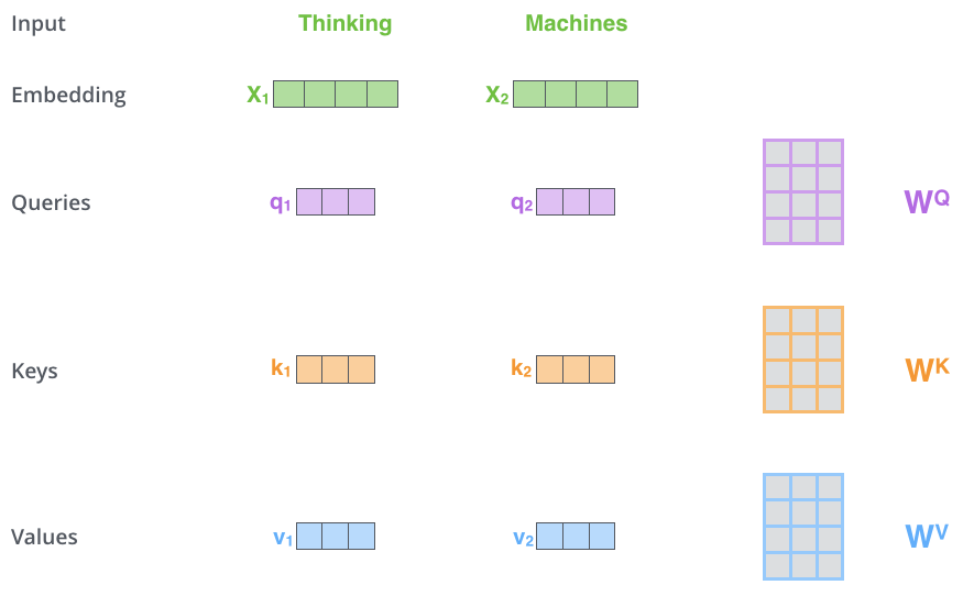
Multiplying x1 by the WQ weight matrix produces q1, the “query” vector associated with that word. We end up creating a “query”, a “key”, and a “value” projection of each word in the input sentence.
What are the “query”, “key”, and “value” vectors?
They’re abstractions that are useful for calculating and thinking about attention. Once you proceed with reading how attention is calculated below, you’ll know pretty much all you need to know about the role each of these vectors plays.
The second step in calculating self-attention is to calculate a score. Say we’re calculating the self-attention for the first word in this example, “Thinking”. We need to score each word of the input sentence against this word. The score determines how much focus to place on other parts of the input sentence as we encode a word at a certain position.
The score is calculated by taking the dot product of the query vector with the key vector of the respective word we’re scoring. So if we’re processing the self-attention for the word in position #1, the first score would be the dot product of q1 and k1. The second score would be the dot product of q1 and k2.
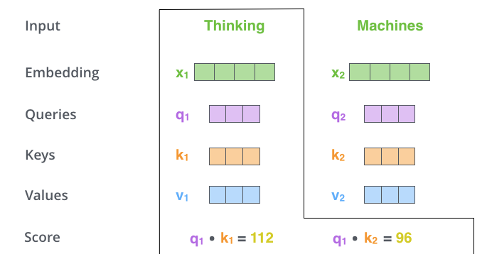
The third and forth steps are to divide the scores by 8 (the square root of the dimension of the key vectors used in the paper — 64. This leads to having more stable gradients. There could be other possible values here, but this is the default), then pass the result through a softmax operation. Softmax normalizes the scores so they’re all positive and add up to 1.
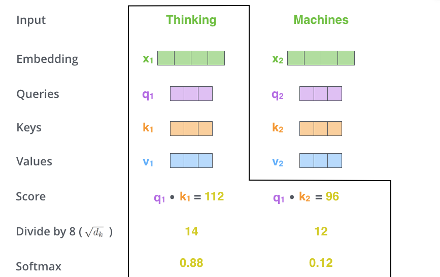
This softmax score determines how much how much each word will be expressed at this position. Clearly the word at this position will have the highest softmax score, but sometimes it’s useful to attend to another word that is relevant to the current word.
The fifth step is to multiply each value vector by the softmax score (in preparation to sum them up). The intuition here is to keep intact the values of the word(s) we want to focus on, and drown-out irrelevant words (by multiplying them by tiny numbers like 0.001, for example).
The sixth step is to sum up the weighted value vectors. This produces the output of the self-attention layer at this position (for the first word).
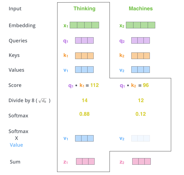
That concludes the self-attention calculation. The resulting vector is one we can send along to the feed-forward neural network. In the actual implementation, however, this calculation is done in matrix form for faster processing. So let’s look at that now that we’ve seen the intuition of the calculation on the word level.
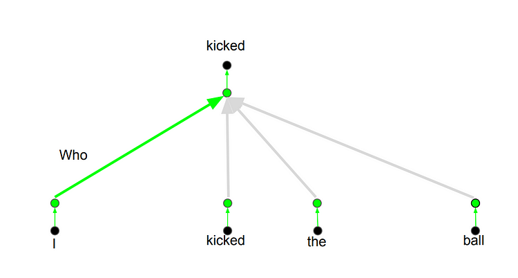
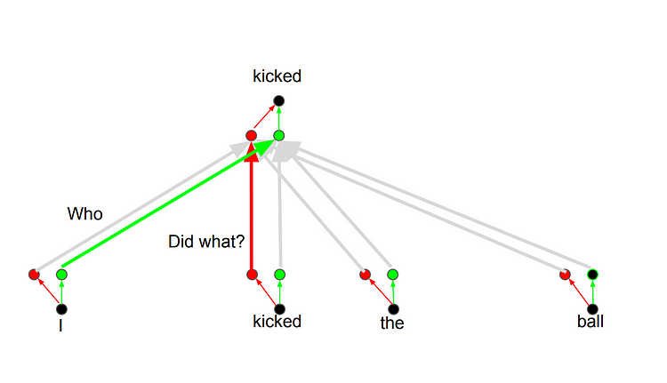
Multihead attention
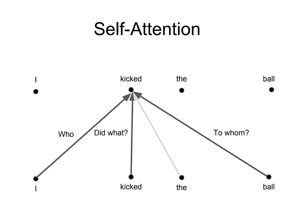
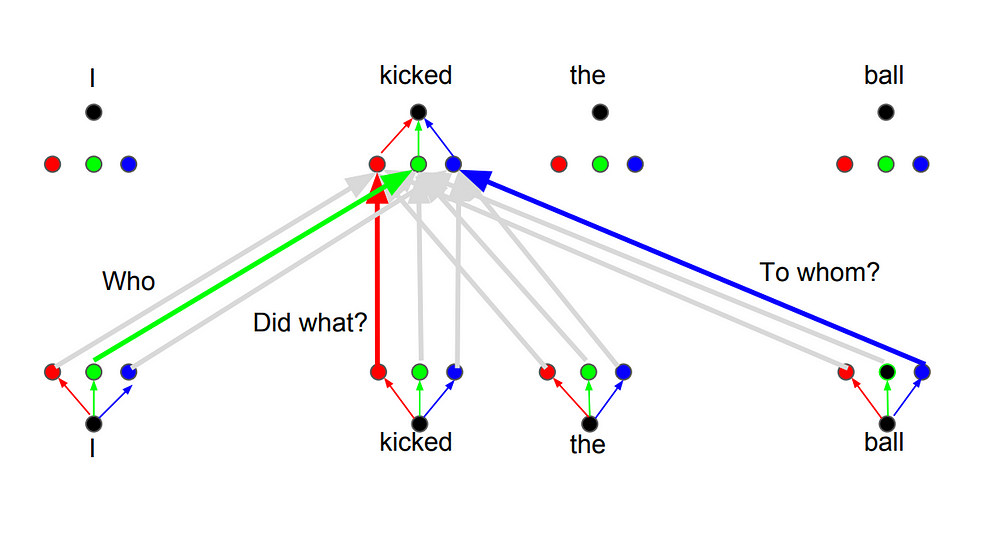
Transformers basically work like that. There are a few other details that make them work better. For example, instead of only paying attention to each other in one dimension, Transformers use the concept of Multihead attention.
The idea behind it is that whenever you are translating a word, you may pay different attention to each word based on the type of question that you are asking. The images below show what that means. For example, whenever you are translating “kicked” in the sentence “I kicked the ball”, you may ask “Who kicked”. Depending on the answer, the translation of the word to another language can change. Or ask other questions, like “Did what?”, etc…
Positional Encoding
Another important step on the Transformer is to add positional encoding when encoding each word. Encoding the position of each word is relevant, since the position of each word is relevant to the translation.
==


 浙公网安备 33010602011771号