聚类(中国大学慕课《机器学习》)ψ(._. )>
1. 无监督学习概述
1.1 监督学习和无监督学习
监督学习
在一个典型的监督学习中,训练集有标签y,我们的目标是找到能够区分正样本和负样本的决策边界,需要据此拟合一个假设函数。
无监督学习
与此不同的是,在无监督学习中,我们的数据没有附带任何标签y,无监督学习主要分为聚类、降维、关联规则、推荐系统等方面。
1.2 主要的无监督学习方法
聚类(Clustering):如何将教室里的学生按爱好、身高划分为5类?降维(Dimensionality Reduction ):如何将将原高维空间中的数据点映射到低维度的空间中?关联规则( Association Rules):很多买尿布的男顾客,同时买了啤酒,可以从中找出什么规律来提高超市销售额?推荐系统(Recommender systems):很多客户经常上网购物,根据他们的浏览商品的习惯,给他们推荐什么商品呢?
1.3 主要聚类算法
K-means、密度聚类、层次聚类。
1.4 聚类算法主要应用
市场细分、文档聚类、图像分割、图像压缩、聚类分析、特征学习或者词典学习、确定犯罪易发地区、保险欺诈检测、公共交通数据分析、IT资产集群、客户细分、识别癌症数据、搜索引擎应用、医疗应用、药物活性预测……
2. K-means聚类
2.1 K-均值算法(K-means)算法概述
K-means算法是一种无监督学习方法,是最普及的聚类算法,算法使用一个没有标签的数据集,然后将数据聚类成不同的组。
K-means算法具有一个迭代过程,在这个过程中,数据集被分组成若干个预定义的不重叠的聚类或子组,使簇的内部点尽可能相似,同时试图保持簇在不同的空间,它将数据点分配给簇,以便簇的质心和数据点之间的平方距离之和最小,在这个位置,簇的质心是簇中数据点的算术平均值。
2.2 闵可夫斯基距离(Minkowski distance)
p=1 曼哈顿距离
p=2 欧氏距离
p= 切比雪夫距离
2.3 K-means算法流程
1、选择K个点作为初始质心。
2、将每个点指派到最近的质心,形成K个簇。
3、对于上一步聚类的结果,进行平均计算,得出该簇的新的聚类中心。
4、重复上述两步/直到迭代结束:质心不发生变化。
2.4 k-means聚类案例
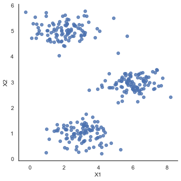
实施和应用K-means到一个简单的二维数据集。
import numpy as np
import pandas as pd
import matplotlib.pyplot as plt
import seaborn as sb
from scipy.io import loadmat
def find_closest_centroids(X, centroids):
    m = X.shape[0]
    k = centroids.shape[0]
    idx = np.zeros(m)

    for i in range(m):
        min_dist = 1000000
        for j in range(k):
            dist = np.sum((X[i, :] - centroids[j, :])**2)
            if dist < min_dist:
                min_dist = dist
                idx[i] = j

    return idx
# 测试这个函数,以确保它的工作正常
data2 = pd.read_csv('data/ex7data2.csv')
data2.head()
X=data2.values
initial_centroids = initial_centroids = np.array([[3, 3], [6, 2], [8, 5]])

idx = find_closest_centroids(X, initial_centroids)
idx[0:3]
# array([0., 2., 1.])
sb.set(context="notebook", style="white")
sb.lmplot(x='X1', y='X2', data=data2, fit_reg=False)
plt.show()
# 计算簇的聚类中心
def compute_centroids(X, idx, k):
    m, n = X.shape
    centroids = np.zeros((k, n))

    for i in range(k):
        indices = np.where(idx == i)
        centroids[i, :] = (np.sum(X[indices, :], axis=1) /
                           len(indices[0])).ravel()

    return centroids
compute_centroids(data2.values, idx, 3)
"""
array([[2.42830111, 3.15792418],
       [5.81350331, 2.63365645],
       [7.11938687, 3.6166844 ]])
"""
def run_k_means(X, initial_centroids, max_iters):
    m, n = X.shape
    k = initial_centroids.shape[0]
    idx = np.zeros(m)
    centroids = initial_centroids

    for i in range(max_iters):
        idx = find_closest_centroids(X, centroids)
        centroids = compute_centroids(X, idx, k)

    return idx, centroids
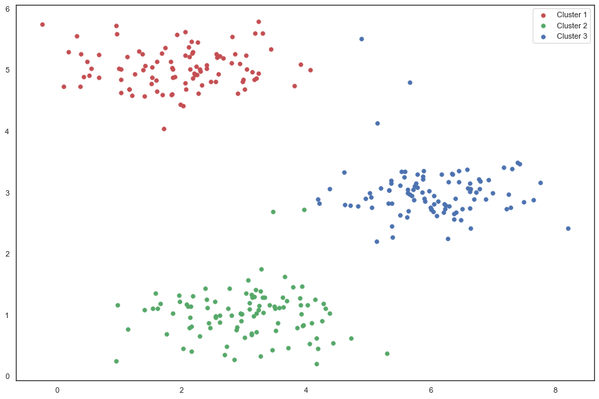
idx, centroids = run_k_means(X, initial_centroids, 10)
cluster1 = X[np.where(idx == 0)[0],:]
cluster2 = X[np.where(idx == 1)[0],:]
cluster3 = X[np.where(idx == 2)[0],:]

fig, ax = plt.subplots(figsize=(15,10))
ax.scatter(cluster1[:,0], cluster1[:,1], s=30, color='r', label='Cluster 1')
ax.scatter(cluster2[:,0], cluster2[:,1], s=30, color='g', label='Cluster 2')
ax.scatter(cluster3[:,0], cluster3[:,1], s=30, color='b', label='Cluster 3')
ax.legend()
plt.show()
我们跳过的一个步骤是初始化聚类中心的过程。 这可以影响算法的收敛。 我们的任务是创建一个选择随机样本并将其用作初始聚类中心的函数。
def init_centroids(X, k):
    m, n = X.shape
    centroids = np.zeros((k, n))
    idx = np.random.randint(0, m, k)

    for i in range(k):
        centroids[i, :] = X[idx[i], :]

    return centroids
init_centroids(X, 3)
"""
array([[3.64846482, 1.62849697],
       [4.60630534, 3.329458  ],
       [5.03611162, 2.92486087]])
"""
2.5 k值的选择(肘部法)
from sklearn.cluster import KMeans

# '利用SSE选择k'
SSE = []  # 存放每次结果的误差平方和
for k in range(1, 9):
    estimator = KMeans(n_clusters=k)  # 构造聚类器
    estimator.fit(data2)
    SSE.append(estimator.inertia_)
X = range(1, 9)

plt.figure(figsize=(15, 10))
plt.xlabel('k')
plt.ylabel('SSE')
plt.plot(X, SSE, 'o-')
plt.show()

可以看出,k=3的时候是肘点,所以,选择k=3
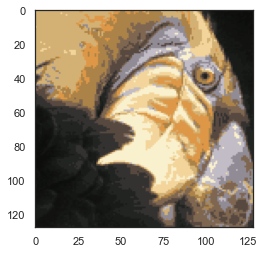
2.6 kmeans图像压缩
使用聚类来找到最具代表性的少数颜色,并使用聚类分配将原始的24位颜色映射到较低维的颜色空间。
from IPython.display import Image
Image(filename='data/bird_small.png')

image_data = loadmat('data/bird_small.mat') # image_data
A = image_data['A']
A.shape #(128, 128, 3)
# normalize value ranges
A = A / 255.

# reshape the array
X = np.reshape(A, (A.shape[0] * A.shape[1], A.shape[2]))
X.shape # (16384, 3)
# randomly initialize the centroids
initial_centroids = init_centroids(X, 16)

# run the algorithm
idx, centroids = run_k_means(X, initial_centroids, 10)

# get the closest centroids one last time
idx = find_closest_centroids(X, centroids)

# map each pixel to the centroid value
X_recovered = centroids[idx.astype(int),:]
X_recovered.shape # (16384, 3)
# reshape to the original dimensions
X_recovered = np.reshape(X_recovered, (A.shape[0], A.shape[1], A.shape[2]))
X_recovered.shape # (128, 128, 3)
plt.imshow(X_recovered)
plt.show()
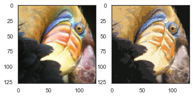
用scikit-learn来实现K-means
from skimage import io
from sklearn.cluster import KMeans#导入kmeans库
import matplotlib.pyplot as plt

# cast to float, you need to do this otherwise the color would be weird after clustring
pic = io.imread('data/bird_small.png') / 255.
# io.imshow(pic)
# plt.show()
# pic.shape # (128, 128, 3)

# serialize data
data = pic.reshape(128*128, 3)
# data.shape # (16384, 3)

model = KMeans(n_clusters=16, n_init=100)
model.fit(data) # KMeans(n_clusters=16, n_init=100)

centroids = model.cluster_centers_
# print(centroids.shape) # (16, 3)
C = model.predict(data)
# print(C.shape) # (16384,)
# centroids[C].shape # (16384, 3)
compressed_pic = centroids[C].reshape((128,128,3))

fig, ax = plt.subplots(1, 2)
ax[0].imshow(pic)
ax[1].imshow(compressed_pic)
plt.show()
3. 密度聚类和层次聚类
3.1 密度聚类
3.1.1 DB-SCAN密度聚类
DBSCAN Density-Based Spatial Clustering of Applications with Noise
DBSCAN是一个比较有代表性的基于密度的聚类算法。
与划分和层次聚类方法不同,它将簇定义为密度相连的点的最大集合,能够把具有足够高密度的区域划分为簇,并可在噪声的空间数据库中发现任意形状的聚类。
3.1.2 DB-SCAN的两个超参数
扫描半径(eps)和最小包含点数(minPts)
来获得簇的数量,而不是猜测簇的数目。
(1)扫描半径(eps):
用于定位点/检查任何点附近密度的距离度量,即扫描半径。
(2)最小包含点数(minPts) :
聚集在一起的最小点数(阈值),该区域被认为是稠密的。
3.1.3 DB-SCAN案例
import numpy as np
import matplotlib.pyplot as plt
from sklearn.cluster import DBSCAN
from sklearn import metrics
from sklearn.datasets import make_blobs
from sklearn.preprocessing import StandardScaler

plt.rcParams['font.sans-serif']=['SimHei'] #用来正常显示中文标签
plt.rcParams['axes.unicode_minus']=False #用来正常显示负号
# 创建样本数据
centers = [[1, 1], [-1, -1], [1, -1]]
X, labels_true = make_blobs(
    n_samples=750, centers=centers, cluster_std=0.4, random_state=0
)

# 标准化数据
X = StandardScaler().fit_transform(X)
# 定义一个 plot_dbscan(MyEps, MiniSample) 函数
# MyEps代表 eps , MiniSample 代表 minPts
def plot_dbscan(MyEps, MiniSample):
    db = DBSCAN(eps=MyEps, min_samples=MiniSample).fit(X)
    core_samples_mask = np.zeros_like(db.labels_, dtype=bool)
    core_samples_mask[db.core_sample_indices_] = True
    labels = db.labels_

    # 标签中的簇数,忽略噪声点(如果存在)。
    n_clusters_ = len(set(labels)) - (1 if -1 in labels else 0)
    n_noise_ = list(labels).count(-1)

    print("估计的簇的数量: %d" % n_clusters_)
    print("估计的噪声点数量: %d" % n_noise_)
    print("同一性(Homogeneity): %0.4f" %
          metrics.homogeneity_score(labels_true, labels))
    print("完整性(Completeness): %0.4f" %
          metrics.completeness_score(labels_true, labels))
    print("V-measure: %0.3f" % metrics.v_measure_score(labels_true, labels))
    print("ARI(Adjusted Rand Index): %0.4f" %
          metrics.adjusted_rand_score(labels_true, labels))
    print("AMI(Adjusted Mutual Information): %0.4f" %
          # metrics.adjusted_mutual_info_score(labels_true, labels))
          # 有一个 warning
          # FutureWarning: The behavior of AMI will change in version 0.22.
          metrics.adjusted_mutual_info_score(labels_true, labels,
                                           average_method='arithmetic'))
    print("轮廓系数(Silhouette Coefficient): %0.4f" %
          metrics.silhouette_score(X, labels))

    # 画出结果

    # 黑色点代表噪声点
    unique_labels = set(labels)
    colors = [
        plt.cm.Spectral(each) for each in np.linspace(0, 1, len(unique_labels))
    ]
    for k, col in zip(unique_labels, colors):
        if k == -1:
            # Black used for noise.
            col = [0, 0, 1, 1]

        class_member_mask = labels == k

        xy = X[class_member_mask & core_samples_mask]
        plt.plot(
            xy[:, 0],
            xy[:, 1],
            "o",
            markerfacecolor=tuple(col),
            markeredgecolor="k",
            markersize=14,
        )

        xy = X[class_member_mask & ~core_samples_mask]
        plt.plot(
            xy[:, 0],
            xy[:, 1],
            "o",
            markerfacecolor=tuple(col),
            markeredgecolor="k",
            markersize=6,
        )

    plt.title("簇的数量为: %d" % n_clusters_, fontsize=18)

#     plt.savefig(str(MyEps) + str(MiniSample) + '.png')#保存图片
    plt.show()
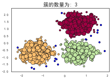
plot_dbscan(0.3, 10)
print('-----------'*3)
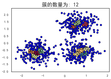
plot_dbscan(0.1, 10)
print('-----------'*3)
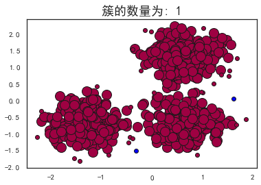
plot_dbscan(0.4, 10)
print('-----------'*3)
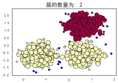
plot_dbscan(0.3, 6)
估计的簇的数量: 3
估计的噪声点数量: 18
同一性(Homogeneity): 0.9530
完整性(Completeness): 0.8832
V-measure: 0.917
ARI(Adjusted Rand Index): 0.9517
AMI(Adjusted Mutual Information): 0.9165
轮廓系数(Silhouette Coefficient): 0.6255
---------------------------------
估计的簇的数量: 12
估计的噪声点数量: 516
同一性(Homogeneity): 0.3128
完整性(Completeness): 0.2489
V-measure: 0.277
ARI(Adjusted Rand Index): 0.0237
AMI(Adjusted Mutual Information): 0.2673
轮廓系数(Silhouette Coefficient): -0.3659
---------------------------------
估计的簇的数量: 1
估计的噪声点数量: 2
同一性(Homogeneity): 0.0010
完整性(Completeness): 0.0586
V-measure: 0.002
ARI(Adjusted Rand Index): -0.0000
AMI(Adjusted Mutual Information): -0.0011
轮廓系数(Silhouette Coefficient): 0.0611
---------------------------------
估计的簇的数量: 2
估计的噪声点数量: 13
同一性(Homogeneity): 0.5365
完整性(Completeness): 0.8263
V-measure: 0.651
ARI(Adjusted Rand Index): 0.5414
AMI(Adjusted Mutual Information): 0.6495
轮廓系数(Silhouette Coefficient): 0.3845
可以看到,当扫描半径 (eps)为0.3,同时最小包含点数(minPts)为10的时候,评价指标最高。
FutureWarning: The behavior of AMI will change in version 0.22. To match the behavior of 'v_measure_score', AMI will use average_method='arithmetic' by default.
print("AMI(Adjusted Mutual Information): %0.4f" %
          metrics.adjusted_mutual_info_score(labels_true, labels))
改为
print("AMI(Adjusted Mutual Information): %0.4f" %
          metrics.adjusted_mutual_info_score(labels_true, labels,
                                           average_method='arithmetic'))
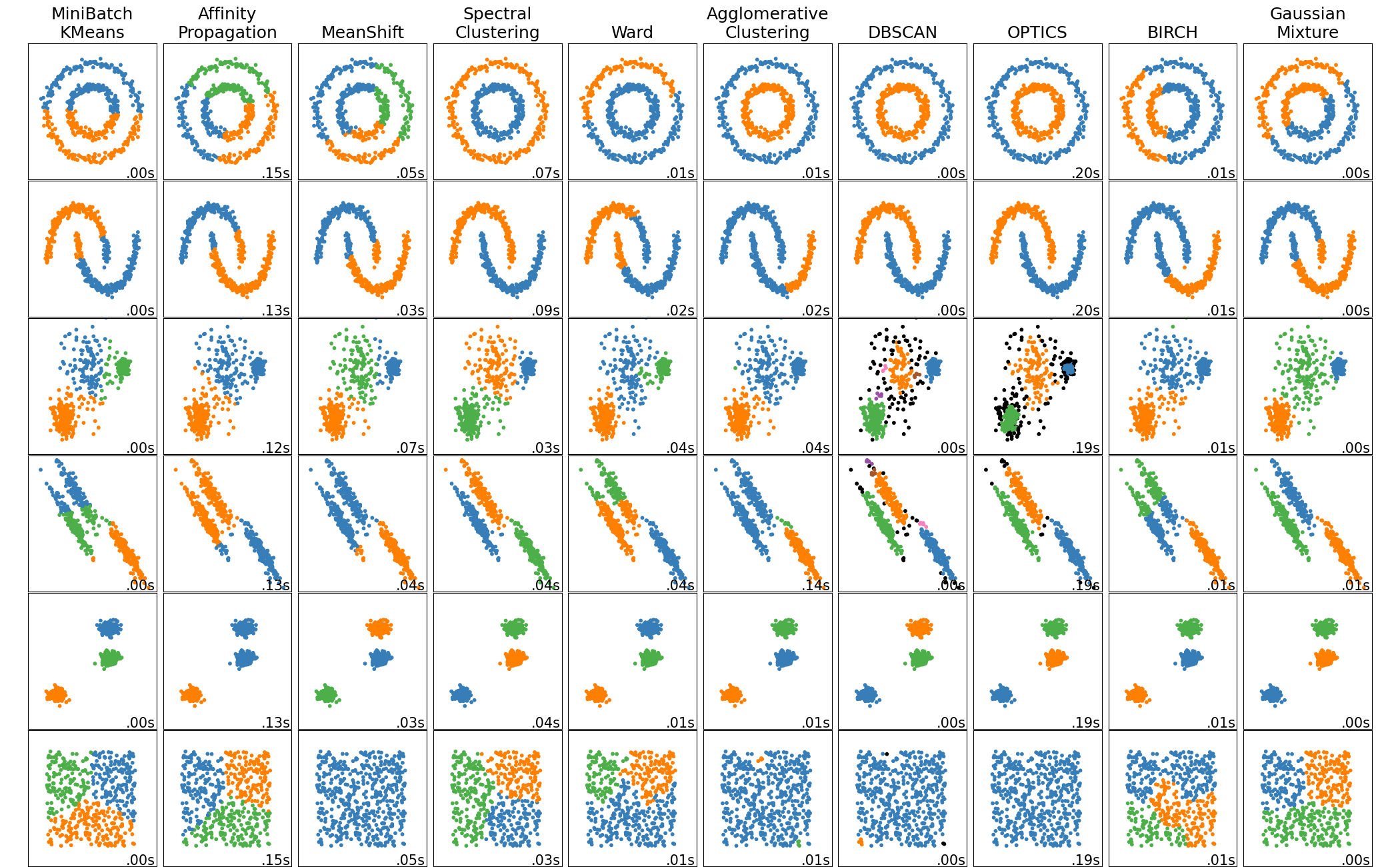
3.1.4 toy数据集上不同聚类算法的比较
Comparing different clustering algorithms on toy datasets
import time
import warnings

import numpy as np
import matplotlib.pyplot as plt

from sklearn import cluster, datasets, mixture
from sklearn.neighbors import kneighbors_graph
from sklearn.preprocessing import StandardScaler
from itertools import cycle, islice

np.random.seed(0)
Generate datasets
n_samples = 500
noisy_circles = datasets.make_circles(n_samples=n_samples, factor=0.5, noise=0.05)
noisy_moons = datasets.make_moons(n_samples=n_samples, noise=0.05)
blobs = datasets.make_blobs(n_samples=n_samples, random_state=8)
no_structure = np.random.rand(n_samples, 2), None

# Anisotropicly distributed data
random_state = 170
X, y = datasets.make_blobs(n_samples=n_samples, random_state=random_state)
transformation = [[0.6, -0.6], [-0.4, 0.8]]
X_aniso = np.dot(X, transformation)
aniso = (X_aniso, y)

# blobs with varied variances
varied = datasets.make_blobs(
    n_samples=n_samples, cluster_std=[1.0, 2.5, 0.5], random_state=random_state
)
Run the clustering and plot
plt.figure(figsize=(9 * 2 + 3, 13))
plt.subplots_adjust(
    left=0.02, right=0.98, bottom=0.001, top=0.95, wspace=0.05, hspace=0.01
)

plot_num = 1

default_base = {
    "quantile": 0.3,
    "eps": 0.3,
    "damping": 0.9,
    "preference": -200,
    "n_neighbors": 3,
    "n_clusters": 3,
    "min_samples": 7,
    "xi": 0.05,
    "min_cluster_size": 0.1,
}

datasets = [
    (
        noisy_circles,
        {
            "damping": 0.77,
            "preference": -240,
            "quantile": 0.2,
            "n_clusters": 2,
            "min_samples": 7,
            "xi": 0.08,
        },
    ),
    (
        noisy_moons,
        {
            "damping": 0.75,
            "preference": -220,
            "n_clusters": 2,
            "min_samples": 7,
            "xi": 0.1,
        },
    ),
    (
        varied,
        {
            "eps": 0.18,
            "n_neighbors": 2,
            "min_samples": 7,
            "xi": 0.01,
            "min_cluster_size": 0.2,
        },
    ),
    (
        aniso,
        {
            "eps": 0.15,
            "n_neighbors": 2,
            "min_samples": 7,
            "xi": 0.1,
            "min_cluster_size": 0.2,
        },
    ),
    (blobs, {"min_samples": 7, "xi": 0.1, "min_cluster_size": 0.2}),
    (no_structure, {}),
]

for i_dataset, (dataset, algo_params) in enumerate(datasets):
    # update parameters with dataset-specific values
    params = default_base.copy()
    params.update(algo_params)

    X, y = dataset

    # normalize dataset for easier parameter selection
    X = StandardScaler().fit_transform(X)

    # estimate bandwidth for mean shift
    bandwidth = cluster.estimate_bandwidth(X, quantile=params["quantile"])

    # connectivity matrix for structured Ward
    connectivity = kneighbors_graph(
        X, n_neighbors=params["n_neighbors"], include_self=False
    )
    # make connectivity symmetric
    connectivity = 0.5 * (connectivity + connectivity.T)

    # ============
    # Create cluster objects
    # ============
    ms = cluster.MeanShift(bandwidth=bandwidth, bin_seeding=True)
    two_means = cluster.MiniBatchKMeans(n_clusters=params["n_clusters"])
    ward = cluster.AgglomerativeClustering(
        n_clusters=params["n_clusters"], linkage="ward", connectivity=connectivity
    )
    spectral = cluster.SpectralClustering(
        n_clusters=params["n_clusters"],
        eigen_solver="arpack",
        affinity="nearest_neighbors",
    )
    dbscan = cluster.DBSCAN(eps=params["eps"])
    optics = cluster.OPTICS(
        min_samples=params["min_samples"],
        xi=params["xi"],
        min_cluster_size=params["min_cluster_size"],
    )
    affinity_propagation = cluster.AffinityPropagation(
        damping=params["damping"], preference=params["preference"], random_state=0
    )
    average_linkage = cluster.AgglomerativeClustering(
        linkage="average",
        affinity="cityblock",
        n_clusters=params["n_clusters"],
        connectivity=connectivity,
    )
    birch = cluster.Birch(n_clusters=params["n_clusters"])
    gmm = mixture.GaussianMixture(
        n_components=params["n_clusters"], covariance_type="full"
    )

    clustering_algorithms = (
        ("MiniBatch\nKMeans", two_means),
        ("Affinity\nPropagation", affinity_propagation),
        ("MeanShift", ms),
        ("Spectral\nClustering", spectral),
        ("Ward", ward),
        ("Agglomerative\nClustering", average_linkage),
        ("DBSCAN", dbscan),
        ("OPTICS", optics),
        ("BIRCH", birch),
        ("Gaussian\nMixture", gmm),
    )

    for name, algorithm in clustering_algorithms:
        t0 = time.time()

        # catch warnings related to kneighbors_graph
        with warnings.catch_warnings():
            warnings.filterwarnings(
                "ignore",
                message="the number of connected components of the "
                + "connectivity matrix is [0-9]{1,2}"
                + " > 1. Completing it to avoid stopping the tree early.",
                category=UserWarning,
            )
            warnings.filterwarnings(
                "ignore",
                message="Graph is not fully connected, spectral embedding"
                + " may not work as expected.",
                category=UserWarning,
            )
            algorithm.fit(X)

        t1 = time.time()
        if hasattr(algorithm, "labels_"):
            y_pred = algorithm.labels_.astype(int)
        else:
            y_pred = algorithm.predict(X)

        plt.subplot(len(datasets), len(clustering_algorithms), plot_num)
        if i_dataset == 0:
            plt.title(name, size=18)

        colors = np.array(
            list(
                islice(
                    cycle(
                        [
                            "#377eb8",
                            "#ff7f00",
                            "#4daf4a",
                            "#f781bf",
                            "#a65628",
                            "#984ea3",
                            "#999999",
                            "#e41a1c",
                            "#dede00",
                        ]
                    ),
                    int(max(y_pred) + 1),
                )
            )
        )
        # add black color for outliers (if any)
        colors = np.append(colors, ["#000000"])
        plt.scatter(X[:, 0], X[:, 1], s=10, color=colors[y_pred])

        plt.xlim(-2.5, 2.5)
        plt.ylim(-2.5, 2.5)
        plt.xticks(())
        plt.yticks(())
        plt.text(
            0.99,
            0.01,
            ("%.2fs" % (t1 - t0)).lstrip("0"),
            transform=plt.gca().transAxes,
            size=15,
            horizontalalignment="right",
        )
        plot_num += 1

plt.show()
AttributeError: module 'sklearn.cluster' has no attribute 'OPTICS'
from sklearn.cluster import OPTICS后ImportError: cannot import name 'OPTICS'
大概是scikit-learn版本问题?
【不知道为什么后来运行就没问题了,难道真的是因为我用pip install -U scikit-learn升级了,但是刚刚明明已经重启内核了还是报错?】
import numpy as np
import matplotlib.pyplot as plt
from matplotlib.colors import ListedColormap
from sklearn.model_selection import train_test_split
from sklearn.preprocessing import StandardScaler
from sklearn.datasets import make_moons, make_circles, make_classification
from sklearn.neural_network import MLPClassifier
from sklearn.neighbors import KNeighborsClassifier
from sklearn.svm import SVC
from sklearn.gaussian_process import GaussianProcessClassifier
from sklearn.gaussian_process.kernels import RBF
from sklearn.tree import DecisionTreeClassifier
from sklearn.ensemble import RandomForestClassifier, AdaBoostClassifier
from sklearn.naive_bayes import GaussianNB
from sklearn.discriminant_analysis import QuadraticDiscriminantAnalysis

h = .02  # step size in the mesh

names = ["Nearest Neighbors", "Linear SVM", "RBF SVM", "Gaussian Process",
         "Decision Tree", "Random Forest", "Neural Net", "AdaBoost",
         "Naive Bayes", "QDA"]

classifiers = [
    KNeighborsClassifier(3),
    SVC(kernel="linear", C=0.025),
    SVC(gamma=2, C=1),
    GaussianProcessClassifier(1.0 * RBF(1.0)),
    DecisionTreeClassifier(max_depth=5),
    RandomForestClassifier(max_depth=5, n_estimators=10, max_features=1),
    MLPClassifier(alpha=1),
    AdaBoostClassifier(),
    GaussianNB(),
    QuadraticDiscriminantAnalysis()]

X, y = make_classification(n_features=2, n_redundant=0, n_informative=2,
                           random_state=1, n_clusters_per_class=1)
rng = np.random.RandomState(2)
X += 2 * rng.uniform(size=X.shape)
linearly_separable = (X, y)

datasets = [make_moons(noise=0.3, random_state=0),
            make_circles(noise=0.2, factor=0.5, random_state=1),
            linearly_separable
            ]

figure = plt.figure(figsize=(27, 9))
i = 1
# iterate over datasets
for ds_cnt, ds in enumerate(datasets):
    # preprocess dataset, split into training and test part
    X, y = ds
    X = StandardScaler().fit_transform(X)
    X_train, X_test, y_train, y_test = \
        train_test_split(X, y, test_size=.4, random_state=42)

    x_min, x_max = X[:, 0].min() - .5, X[:, 0].max() + .5
    y_min, y_max = X[:, 1].min() - .5, X[:, 1].max() + .5
    xx, yy = np.meshgrid(np.arange(x_min, x_max, h),
                         np.arange(y_min, y_max, h))

    # just plot the dataset first
    cm = plt.cm.RdBu
    cm_bright = ListedColormap(['#FF0000', '#0000FF'])
    ax = plt.subplot(len(datasets), len(classifiers) + 1, i)
    if ds_cnt == 0:
        ax.set_title("Input data")
    # Plot the training points
    ax.scatter(X_train[:, 0], X_train[:, 1], c=y_train, cmap=cm_bright,
               edgecolors='k')
    # Plot the testing points
    ax.scatter(X_test[:, 0], X_test[:, 1], c=y_test, cmap=cm_bright, alpha=0.6,
               edgecolors='k')
    ax.set_xlim(xx.min(), xx.max())
    ax.set_ylim(yy.min(), yy.max())
    ax.set_xticks(())
    ax.set_yticks(())
    i += 1

    # iterate over classifiers
    for name, clf in zip(names, classifiers):
        ax = plt.subplot(len(datasets), len(classifiers) + 1, i)
        clf.fit(X_train, y_train)
        score = clf.score(X_test, y_test)

        # Plot the decision boundary. For that, we will assign a color to each
        # point in the mesh [x_min, x_max]x[y_min, y_max].
        if hasattr(clf, "decision_function"):
            Z = clf.decision_function(np.c_[xx.ravel(), yy.ravel()])
        else:
            Z = clf.predict_proba(np.c_[xx.ravel(), yy.ravel()])[:, 1]

        # Put the result into a color plot
        Z = Z.reshape(xx.shape)
        ax.contourf(xx, yy, Z, cmap=cm, alpha=.8)

        # Plot the training points
        ax.scatter(X_train[:, 0], X_train[:, 1], c=y_train, cmap=cm_bright,
                   edgecolors='k')
        # Plot the testing points
        ax.scatter(X_test[:, 0], X_test[:, 1], c=y_test, cmap=cm_bright,
                   edgecolors='k', alpha=0.6)

        ax.set_xlim(xx.min(), xx.max())
        ax.set_ylim(yy.min(), yy.max())
        ax.set_xticks(())
        ax.set_yticks(())
        if ds_cnt == 0:
            ax.set_title(name)
        ax.text(xx.max() - .3, yy.min() + .3, ('%.2f' % score).lstrip('0'),
                size=15, horizontalalignment='right')
        i += 1

plt.tight_layout()
plt.show()
# 0.20.4版本
3.2 层次聚类
层次聚类假设簇之间存在层次结构,将样本聚到层次化的簇中。
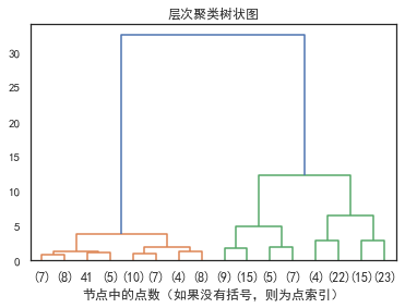
3.2.0 层次聚类树状图
import numpy as np
import matplotlib.pyplot as plt
from scipy.cluster.hierarchy import dendrogram
from sklearn.datasets import load_iris
from sklearn.cluster import AgglomerativeClustering

plt.rcParams['font.sans-serif']=['SimHei'] #用来正常显示中文标签
plt.rcParams['axes.unicode_minus']=False #用来正常显示负号
def plot_dendrogram(model, **kwargs):
    # 创建链接矩阵,然后绘制树状图

    # 创建每个节点下的样本计数
    counts = np.zeros(model.children_.shape[0])
    n_samples = len(model.labels_)
    for i, merge in enumerate(model.children_):
        current_count = 0
        for child_idx in merge:
            if child_idx < n_samples:
                current_count += 1  # leaf node
            else:
                current_count += counts[child_idx - n_samples]
        counts[i] = current_count

    linkage_matrix = np.column_stack(
        [model.children_, model.distances_, counts]
    ).astype(float)

    # 绘制相应的树状图
    dendrogram(linkage_matrix, **kwargs)
iris = load_iris()
X = iris.data

# 设置距离阈值=0可确保计算完整的树。
model = AgglomerativeClustering(distance_threshold=0, n_clusters=None)
model = model.fit(X)

plt.title("层次聚类树状图")
# 绘制树状图的前三级
plot_dendrogram(model, truncate_mode="level", p=3)
plt.xlabel("节点中的点数(如果没有括号,则为点索引)")
plt.show()
层次聚类又有聚合聚类(自下而上)、分裂聚类(自上而下)两种方法。
如果一个聚类方法假定一个样本只能属于一个簇,或簇的交集为空集,那么该方法称为硬聚类方法。 如果一个样本可以属于多个簇,或簇的交集不为空集,那么该方法称为软聚类方法。
3.2.1 聚合聚类
- 开始将每个样本各自分到一个簇;
- 之后将相距
最近的两簇合并,建立一个新的簇; - 重复此操作直到满足停止条件;
- 得到层次化的类别。
3.2.2 分裂聚类
- 开始将所有样本分到一个簇;
- 之后将已有类中
相距最远的样本分到两个新的簇; - 重复此操作直到满足停止条件;
- 得到层次化的类别。
4. 聚类的评价指标
4.1 均一性:p
类似于精确率,一个簇中只包含一个类别的样本,则满足均一性。其实也可以认为就是正确率(每个聚簇中正确分类的样本数占该聚簇总样本数的比例和)
4.2 完整性:r
类似于召回率,同类别样本被归类到相同簇中,则满足完整性;(每个聚簇中正确分类的羊本数占该类型的总样本数比例的和)
V-measure:V
均一性和完整性的加权平均
4.3 轮廓系数
样本i的轮廓系数
-1≤s(i)≤1
- 簇内不相似度:计算样本i到同簇其它样本的平均距离为a(i),应尽可能小。
- 簇间不相似度:计算样本i到其它簇Cj的所有样本的平均距离 bij,应尽可能大。
轮廓系数s(i)值越接近1表示样本i聚类越合理,越接近-1表示样本i应该分类到另外的簇中,近似为0,表示样本i应该在边界上;所有样本的s(i)的均值被成为聚类结果的轮廓系数。
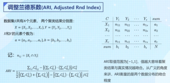
4.4 调整兰德系数:ARI
5. 一些聚类案例
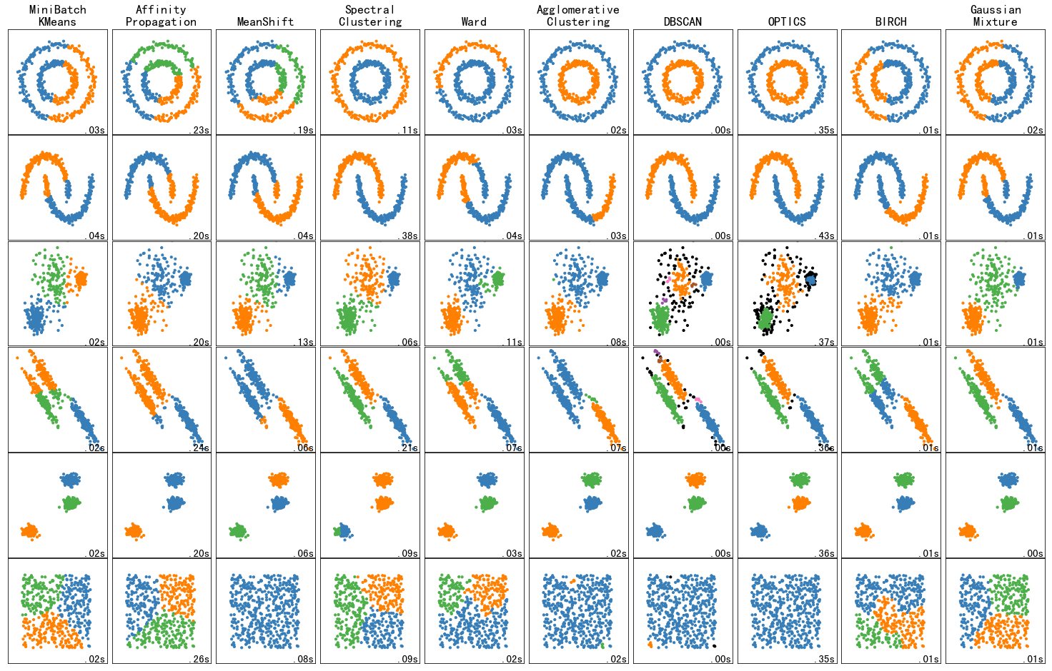
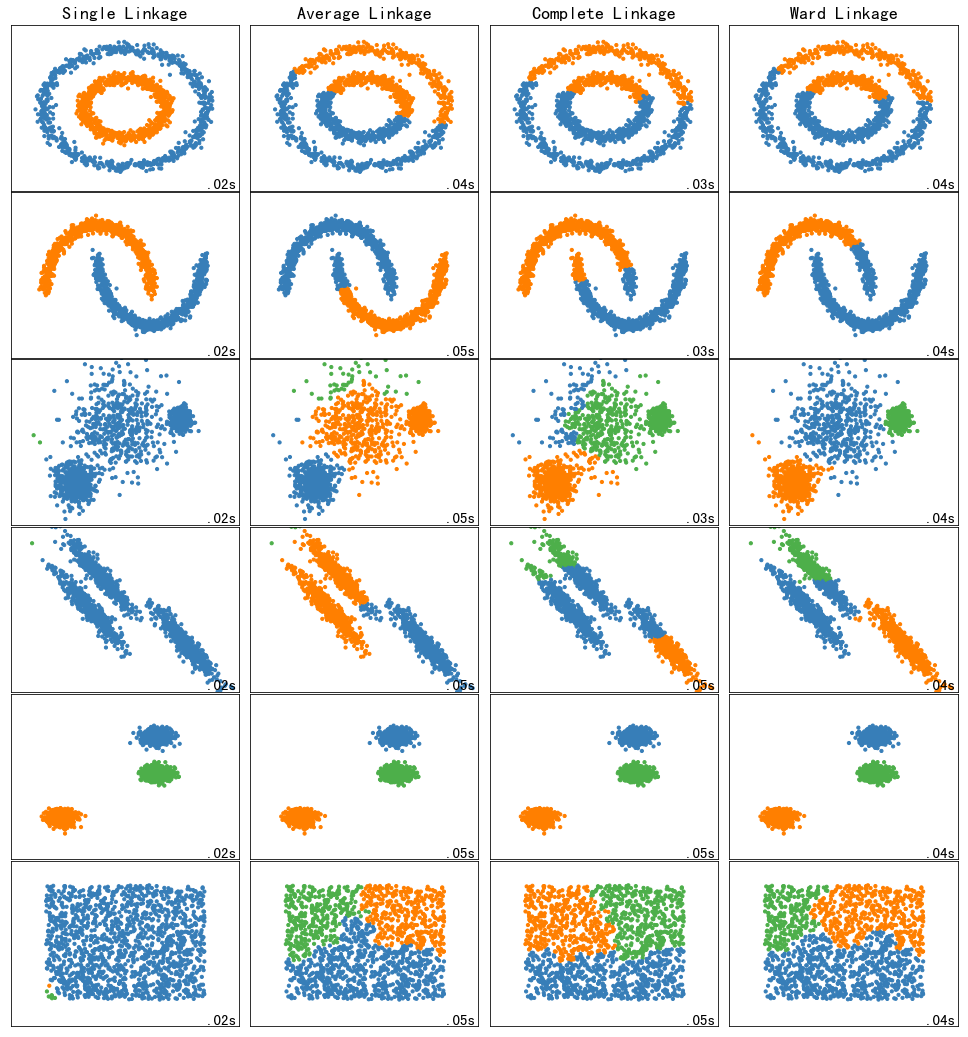
5.1 toy数据集上不同层次链接方法的比较
Comparing different hierarchical linkage methods on toy datasets
import time
import warnings

import numpy as np
import matplotlib.pyplot as plt

from sklearn import cluster, datasets
from sklearn.preprocessing import StandardScaler
from itertools import cycle, islice

np.random.seed(0)
Generate datasets
n_samples = 1500
noisy_circles = datasets.make_circles(n_samples=n_samples, factor=0.5, noise=0.05)
noisy_moons = datasets.make_moons(n_samples=n_samples, noise=0.05)
blobs = datasets.make_blobs(n_samples=n_samples, random_state=8)
no_structure = np.random.rand(n_samples, 2), None

# Anisotropicly distributed data
random_state = 170
X, y = datasets.make_blobs(n_samples=n_samples, random_state=random_state)
transformation = [[0.6, -0.6], [-0.4, 0.8]]
X_aniso = np.dot(X, transformation)
aniso = (X_aniso, y)

# blobs with varied variances
varied = datasets.make_blobs(
    n_samples=n_samples, cluster_std=[1.0, 2.5, 0.5], random_state=random_state
)
Run the clustering and plot
# Set up cluster parameters
plt.figure(figsize=(9 * 1.3 + 2, 14.5))
plt.subplots_adjust(
    left=0.02, right=0.98, bottom=0.001, top=0.96, wspace=0.05, hspace=0.01
)

plot_num = 1

default_base = {"n_neighbors": 10, "n_clusters": 3}

datasets = [
    (noisy_circles, {"n_clusters": 2}),
    (noisy_moons, {"n_clusters": 2}),
    (varied, {"n_neighbors": 2}),
    (aniso, {"n_neighbors": 2}),
    (blobs, {}),
    (no_structure, {}),
]

for i_dataset, (dataset, algo_params) in enumerate(datasets):
    # update parameters with dataset-specific values
    params = default_base.copy()
    params.update(algo_params)

    X, y = dataset

    # normalize dataset for easier parameter selection
    X = StandardScaler().fit_transform(X)

    # ============
    # Create cluster objects
    # ============
    ward = cluster.AgglomerativeClustering(
        n_clusters=params["n_clusters"], linkage="ward"
    )
    complete = cluster.AgglomerativeClustering(
        n_clusters=params["n_clusters"], linkage="complete"
    )
    average = cluster.AgglomerativeClustering(
        n_clusters=params["n_clusters"], linkage="average"
    )
    single = cluster.AgglomerativeClustering(
        n_clusters=params["n_clusters"], linkage="single"
    )

    clustering_algorithms = (
        ("Single Linkage", single),
        ("Average Linkage", average),
        ("Complete Linkage", complete),
        ("Ward Linkage", ward),
    )

    for name, algorithm in clustering_algorithms:
        t0 = time.time()

        # catch warnings related to kneighbors_graph
        with warnings.catch_warnings():
            warnings.filterwarnings(
                "ignore",
                message="the number of connected components of the "
                + "connectivity matrix is [0-9]{1,2}"
                + " > 1. Completing it to avoid stopping the tree early.",
                category=UserWarning,
            )
            algorithm.fit(X)

        t1 = time.time()
        if hasattr(algorithm, "labels_"):
            y_pred = algorithm.labels_.astype(int)
        else:
            y_pred = algorithm.predict(X)

        plt.subplot(len(datasets), len(clustering_algorithms), plot_num)
        if i_dataset == 0:
            plt.title(name, size=18)

        colors = np.array(
            list(
                islice(
                    cycle(
                        [
                            "#377eb8",
                            "#ff7f00",
                            "#4daf4a",
                            "#f781bf",
                            "#a65628",
                            "#984ea3",
                            "#999999",
                            "#e41a1c",
                            "#dede00",
                        ]
                    ),
                    int(max(y_pred) + 1),
                )
            )
        )
        plt.scatter(X[:, 0], X[:, 1], s=10, color=colors[y_pred])

        plt.xlim(-2.5, 2.5)
        plt.ylim(-2.5, 2.5)
        plt.xticks(())
        plt.yticks(())
        plt.text(
            0.99,
            0.01,
            ("%.2fs" % (t1 - t0)).lstrip("0"),
            transform=plt.gca().transAxes,
            size=15,
            horizontalalignment="right",
        )
        plot_num += 1

plt.show()
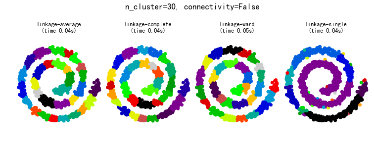
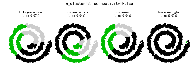
5.2 有结构和无结构的聚集聚类
Agglomerative clustering with and without structure
import time
import matplotlib.pyplot as plt
import numpy as np

from sklearn.cluster import AgglomerativeClustering
from sklearn.neighbors import kneighbors_graph

# Generate sample data
n_samples = 1500
np.random.seed(0)
t = 1.5 * np.pi * (1 + 3 * np.random.rand(1, n_samples))
x = t * np.cos(t)
y = t * np.sin(t)

X = np.concatenate((x, y))
X += 0.7 * np.random.randn(2, n_samples)
X = X.T

# Create a graph capturing local connectivity. Larger number of neighbors
# will give more homogeneous clusters to the cost of computation
# time. A very large number of neighbors gives more evenly distributed
# cluster sizes, but may not impose the local manifold structure of
# the data
knn_graph = kneighbors_graph(X, 30, include_self=False)

for connectivity in (None, knn_graph):
    for n_clusters in (30, 3):
        plt.figure(figsize=(10, 4))
        for index, linkage in enumerate(("average", "complete", "ward", "single")):
            plt.subplot(1, 4, index + 1)
            model = AgglomerativeClustering(
                linkage=linkage, connectivity=connectivity, n_clusters=n_clusters
            )
            t0 = time.time()
            model.fit(X)
            elapsed_time = time.time() - t0
            plt.scatter(X[:, 0], X[:, 1], c=model.labels_, cmap=plt.cm.nipy_spectral)
            plt.title(
                "linkage=%s\n(time %.2fs)" % (linkage, elapsed_time),
                fontdict=dict(verticalalignment="top"),
            )
            plt.axis("equal")
            plt.axis("off")

            plt.subplots_adjust(bottom=0, top=0.83, wspace=0, left=0, right=1)
            plt.suptitle(
                "n_cluster=%i, connectivity=%r"
                % (n_clusters, connectivity is not None),
                size=17,
            )

plt.show()


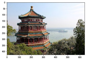
5.3 使用K-means的颜色量化
Color Quantization using K-Means
china=load_sample_image('china.jpg')
plt.imshow(china)
plt.show()
import numpy as np
import matplotlib.pyplot as plt
from sklearn.cluster import KMeans
from sklearn.metrics import pairwise_distances_argmin
from sklearn.datasets import load_sample_image # china图片是这的
from sklearn.utils import shuffle
from time import time

n_colors = 64

# Load the Summer Palace photo
china = load_sample_image("china.jpg")

# Convert to floats instead of the default 8 bits integer coding. Dividing by
# 255 is important so that plt.imshow behaves works well on float data (need to
# be in the range [0-1])
china = np.array(china, dtype=np.float64) / 255

# Load Image and transform to a 2D numpy array.
w, h, d = original_shape = tuple(china.shape)
assert d == 3
image_array = np.reshape(china, (w * h, d))

print("Fitting model on a small sub-sample of the data")
t0 = time()
image_array_sample = shuffle(image_array, random_state=0, n_samples=1_000)
kmeans = KMeans(n_clusters=n_colors, random_state=0).fit(image_array_sample)
print(f"done in {time() - t0:0.3f}s.")

# Get labels for all points
print("Predicting color indices on the full image (k-means)")
t0 = time()
labels = kmeans.predict(image_array)
print(f"done in {time() - t0:0.3f}s.")


codebook_random = shuffle(image_array, random_state=0, n_samples=n_colors)
print("Predicting color indices on the full image (random)")
t0 = time()
labels_random = pairwise_distances_argmin(codebook_random, image_array, axis=0)
print(f"done in {time() - t0:0.3f}s.")


def recreate_image(codebook, labels, w, h):
    """Recreate the (compressed) image from the code book & labels"""
    return codebook[labels].reshape(w, h, -1)


# Display all results, alongside original image
plt.figure(1)
plt.clf()
plt.axis("off")
plt.title("Original image (96,615 colors)")
plt.imshow(china)

plt.figure(2)
plt.clf()
plt.axis("off")
plt.title(f"Quantized image ({n_colors} colors, K-Means)")
plt.imshow(recreate_image(kmeans.cluster_centers_, labels, w, h))

plt.figure(3)
plt.clf()
plt.axis("off")
plt.title(f"Quantized image ({n_colors} colors, Random)")
plt.imshow(recreate_image(codebook_random, labels_random, w, h))
plt.show()


【推荐】国内首个AI IDE,深度理解中文开发场景,立即下载体验Trae
【推荐】编程新体验,更懂你的AI,立即体验豆包MarsCode编程助手
【推荐】抖音旗下AI助手豆包,你的智能百科全书,全免费不限次数
【推荐】轻量又高性能的 SSH 工具 IShell:AI 加持,快人一步
· 25岁的心里话
· 闲置电脑爆改个人服务器(超详细) #公网映射 #Vmware虚拟网络编辑器
· 零经验选手,Compose 一天开发一款小游戏!
· 通过 API 将Deepseek响应流式内容输出到前端
· 因为Apifox不支持离线,我果断选择了Apipost!