机器学习:逻辑回归(损失函数及其梯度推导、代码实现)

一、线性模型预测一个样本的损失量

  • 损失量:模型对样本的预测结果和该样本对应的实际结果的差距;

 1)为什么会想到用 y = -log(x) 函数?

  • (该函数称为 惩罚函数:预测结果与实际值的偏差越大,惩罚越大


  1. y = 1(p ≥ 0.5)时,cost = -log(p),p 越小,样本发生概率越小(最小为 0),则损失函数越大,分类预测值和实际值的偏差越大;相反,p 越大,样本发生概率越大(最大为 0.5),则损失函数越小,则预测值和实际值的偏差越小;
  2. y = 0(p ≤ 0.5)时,cost = -log(1-p),p 越小,样本发生概率越小(最小为 0.5),则损失函数越大,分类预测值和实际值的偏差越大;相反,p 越大,样本发生概率越大(最大为 1),则损失函数越小,则预测值和实际值的偏差越小;


 2)求一个样本的损失量

  • 由于逻辑回归解决的是分类问题,而且是二分类,因此定义损失函数时也要有两类
  • 惩罚函数变形:
  • 惩罚函数作用:计算预测结果针对实际值的损失量;
  1. 已知样本发生的概率 p(也可以相应求出预测值),以及该样本的实际分类结果,得出此次预测结果针对真值的损失量是多少;


二、求数据集的损失函数

  • 模型变形,得到数据集的损失函数数据集中的所有样本的损失值的和


  • 最终的损失函数模型
  1. 该模型不能优化成简单的数学表达式(或者说是正规方程解:线性回归算法找那个的fit_normal() 方法),只能使用梯度下降法求解;
  2. 该函数为凸函数,没有局部最优解,只存在全局最优解;


三、逻辑回归损失函数的梯度

  • 损失函数:


 1)σ(t) 函数的导数


 2)log(σ(t)) 函数的导数


  • 变形:


 3)log(1 - σ(t)) 函数的导数


 3)对损失函数 J(θ) 的其中某一项(第 i 行,第 j 列)求导

  1. 两式相加:


 5)损失函数 J(θ) 的梯度


  • 与线性回归梯度对比
  1. 两者的预测值 ý 不同


  • 梯度向量化处理


四、代码实现逻辑回归算法

  • 逻辑回归算法是在线性回归算法的基础上演变的;

 1)代码

  • import numpy as np
    from .metrics import accuracy_score
    
    # accuracy_score方法:查看准确率
    
    class LogisticRegression:
    
        def __init__(self):
            """初始化Logistic Regression模型"""
            self.coef_ = None
            self.intercept_ = None
            self._theta = None
    
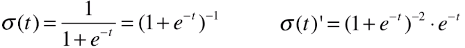
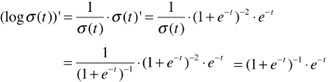
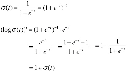
        def _sigmiod(self, t):
            """函数名首部为'_',表明该函数为私有函数,其它模块不能调用"""
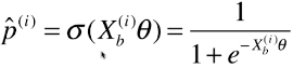
            return 1. / (1. + np.exp(-t))
    
        def fit(self, X_train, y_train, eta=0.01, n_iters=1e4):
            """根据训练数据集X_train, y_train, 使用梯度下降法训练Logistic Regression模型"""
            assert X_train.shape[0] == y_train.shape[0], \
                "the size of X_train must be equal to the size of y_train"
    
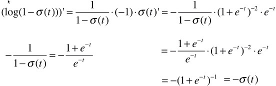
            def J(theta, X_b, y):
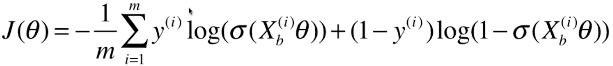
                y_hat = self._sigmiod(X_b.dot(theta))
                try:
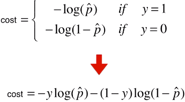
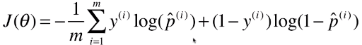
                    return - np.sum(y*np.log(y_hat) + (1-y)*np.log(1-y_hat)) / len(y)
                except:
                    return float('inf')
    
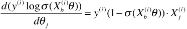
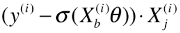
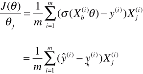
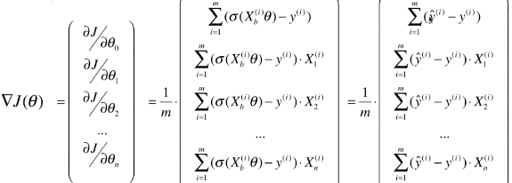
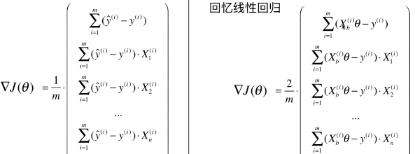
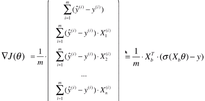
            def dJ(theta, X_b, y):
                return X_b.T.dot(self._sigmiod(X_b.dot(theta)) - y) / len(X_b)
    
            def gradient_descent(X_b, y, initial_theta, eta, n_iters=1e4, epsilon=1e-8):
    
                theta = initial_theta
                cur_iter = 0
    
                while cur_iter < n_iters:
                    gradient = dJ(theta, X_b, y)
                    last_theta = theta
                    theta = theta - eta * gradient
                    if (abs(J(theta, X_b, y) - J(last_theta, X_b, y)) < epsilon):
                        break
    
                    cur_iter += 1
    
                return theta
    
            X_b = np.hstack([np.ones((len(X_train), 1)), X_train])
            initial_theta = np.zeros(X_b.shape[1])
            self._theta = gradient_descent(X_b, y_train, initial_theta, eta, n_iters)
    
            self.intercept_ = self._theta[0]
            self.coef_ = self._theta[1:]
    
            return self
    
        def predict_proda(self, X_predict):
            """给定待预测数据集X_predict,返回 X_predict 中的样本的发生的概率向量"""
            assert self.intercept_ is not None and self.coef_ is not None, \
                "must fit before predict!"
            assert X_predict.shape[1] == len(self.coef_), \
                "the feature number of X_predict must be equal to X_train"
    
            X_b = np.hstack([np.ones((len(X_predict), 1)), X_predict])
            return self._sigmiod(X_b.dot(self._theta))
    
        def predict(self, X_predict):
            """给定待预测数据集X_predict,返回表示X_predict的分类结果的向量"""
            assert self.intercept_ is not None and self.coef_ is not None, \
                "must fit before predict!"
            assert X_predict.shape[1] == len(self.coef_), \
                "the feature number of X_predict must be equal to X_train"
    
            proda = self.predict_proda(X_predict)
            # proda:单个待预测样本的发生概率
            # proda >= 0.5:返回元素为布尔类型的向量;
            # np.array(proda >= 0.5, dtype='int'):将布尔数据类型的向量转化为元素为 int 型的数组,则该数组中的 0 和 1 代表两种不同的分类类别;
            return np.array(proda >= 0.5, dtype='int')
    
        def score(self, X_test, y_test):
            """根据测试数据集 X_test 和 y_test 确定当前模型的准确度"""
    
            y_predict = self.predict(X_test)
            # 分类问题的化,查看标准是分类的准确度:accuracy_score(y_test, y_predict)
            return accuracy_score(y_test, y_predict)
    
        def __repr__(self):
            """实例化类之后,输出显示 LogisticRegression()"""
            return "LogisticRegression()"


 2)使用自己的算法(Jupyter NoteBook 中使用)

  • 代码
    import numpy as np
    import matplotlib.pyplot as plt
    from sklearn import datasets
    
    iris = datasets.load_iris()
    X = iris.data
    y = iris.target
    X = X[y<2, :2]
    y = y[y<2]
    
    
    from playML.train_test_split import train_test_split
    X_train, X_test, y_train, y_test
    = train_test_split(X, y, seed=666)
    from playML.LogisticRegression import LogisticRegression log_reg = LogisticRegression() log_reg.fit(X_train, y_train) log_reg.score(X_test, y_test) # 输出:1.0 # 查看测试数据集的样本发生的概率 log_reg.predict_proda(X_test) # 输出:array([0.92972035, 0.98664939, 0.14852024, 0.17601199, 0.0369836 , 0.0186637 , 0.04936918, 0.99669244, 0.97993941, 0.74524655, 0.04473194, 0.00339285, 0.26131273, 0.0369836 , 0.84192923, 0.79892262, 0.82890209, 0.32358166, 0.06535323, 0.20735334])


posted @ 2018-07-15 18:31  何永灿  阅读(5899)  评论(1编辑  收藏  举报