命令行记录-机器学习(scikit-learn)包
https://sklearn.apachecn.org/
1.离群值(点)识别
离群值(outlier)是指在一组数据中出现的与大部分数值相比差异较大的个别值。
关键问题:差异有多大、如何判断?
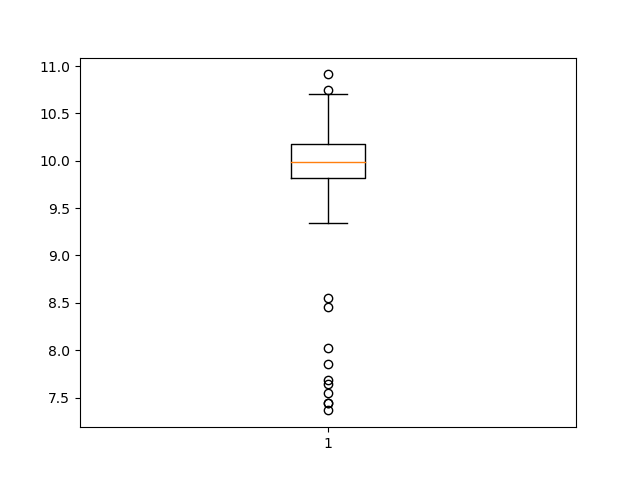
( 1)利用直方图或盒状图直接判断
置信水平, 显著偏离直方图主体频数区域的数值;或者距离盒状图的箱体(第 1 个四分位数和第 3 四分位数)过远,如超出3倍的IQR距离。
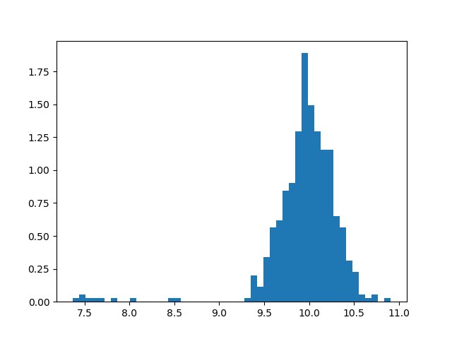
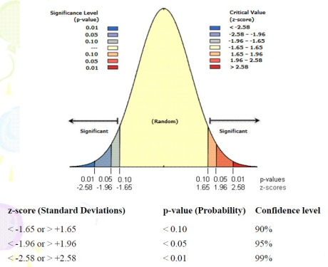
( 2)若一组数据符合某种分布( scipy.stats),则可用置信区间或显著水平判断
#p-value 和 z-score 关系
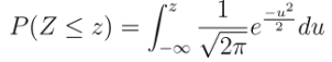
P 值不是给定样本结果时原假设为真的概率,而是给定原假设为真时样本结果出现的概率。 计算出 P 值后,将给定的显著性水平 α 与 P 值比较,就可作出检验的结论:如果 α > P值,则在显著性水平 α 下拒绝原假设。如果 α ≤ P 值,则在显著性水平 α 下接受原假设。
# pdf - Probability density function
# cdf - Cumulative distribution function
# ppf - Percent point function (inverse of cdf — percentiles)
#z-score = ppf(p-value), p-value = cdf(z-score)
 1 #(2)若一组数据符合某种分布(scipy.stats),则可用置信区间或显著水平判断
 2 #
 3 import numpy as np
 4 import matplotlib.mlab as mlab
 5 import matplotlib.pyplot as plt
 6 from scipy.stats import norm,gengamma,gamma
 7
 8 # 模拟一组带噪音的数据
 9 mu, sigma = 10, 0.25
10 x = np.random.normal(mu, sigma, 500) #samples
11 t = np.random.normal(8, 0.5, 10) #outliers
12 x[:10] = t
13
14 #假设已知该组数据是正态(高斯)分布, 参数估计获得其参数
15 #mu_,sigma_ = rv_continuous.fit(norm, x)
16 mu_,sigma_ = norm.fit(x)
17 rv = norm(mu_,sigma_)
18
19 #Pr(c1<=μ<=c2)=1-α
20 #alpha=0.05; confidence level, 1-α; confidence interval [c1, c2]
21 #显著性水平 alpha=0.05,置信水平( 1-0.05=95%), 置信区间[c1, c2]
22 #c1, c2= norm.interval(0.95, loc=mu_, scale=sigma_)
23 #c1, c2= rv.interval(0.95) #Percent point function (inverse of cdf — percentiles)
24
25 c1= rv.ppf(0.025) #置信极限值,左右两边的z值,小于9.2,大于10.69都是离群值
26 c2= rv.ppf(0.975)
27 z_score = c1
28 p_value =rv.cdf(z_score) #Cumulative distribution function
29
30 #离群值
31 xmin,xmax = c1,c2
32 inx = np.where( (x<xmin)+(x>xmax) > 0 )#这句代码是什么意思?
33 t_ = x[inx]
34
35 #图示
36 n, bins, patches = plt.hist(x,50,density=1)
37 y = norm.pdf(bins, mu, sigma)
38 y_ = norm.pdf(bins, mu_, sigma_)
39 plt.plot(bins, y, 'g--')
40 plt.plot(bins, y_, 'r--')
41 plt.plot([xmin,xmin],[0,1.5], 'r--')
42 plt.plot([xmax,xmax],[0,1.5], 'r--')
43 plt.show()

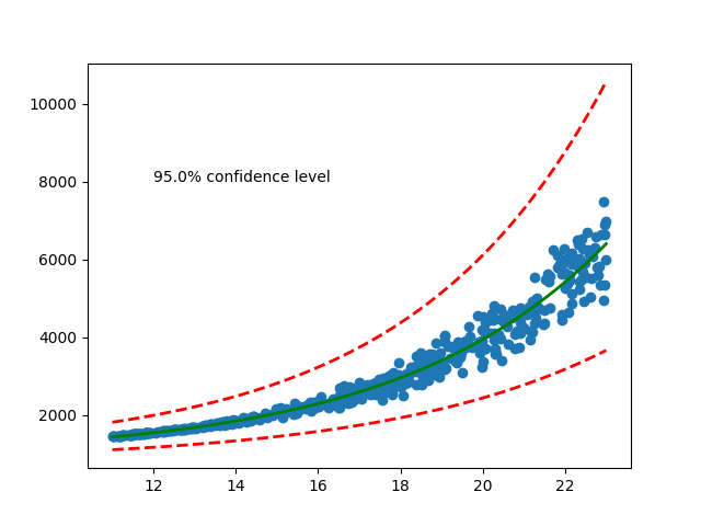
( 3) 给定一组样本数据符合一特定数学模型, 计算并画出其 confidence interval (bands)
非线性拟合方程
 1 #( 3) 给定一组样本数据符合一特定数学模型, 计算并画出其 confidence interval (bands)
 2 #
 3 from scipy.optimize import curve_fit
 4 from scipy import stats
 5 import matplotlib.pyplot as plt
 6 import numpy as np
 7
 8 #y = a*ebx + c
 9 def func(x, a, b, c):
10     '''Exponential 3-param function.'''
11     return a * np.exp(b * x) + c
12
13 # Generating a dataset
14 n = 500
15 a,b,c = 50,0.2,1000
16 x = 11 + np.random.random(n)*12
17 #y= func(x,a,b,c)
18 y = a * np.exp(b * x) + c + (np.random.random(n)-0.2)*10*(x-11)**2 +\
19     (np.random.random(n)-0.5)*10*(x-11)**2#加噪音
20
21 # Define confidence level
22 ci = 0.95
23 # Convert to percentile point of the normal distribution.
24 # See: https://en.wikipedia.org/wiki/Standard_score
25 pp = (1. + ci) / 2.
26 # Convert to number of standard deviations.
27 nstd = stats.norm.ppf(pp)#对应n倍的lambda,一会要加在a,b,c的系数上
28
29 # Find best fit.
30 popt, pcov = curve_fit(func, x, y, p0=(20,1,1))
31 # Standard deviation errors on the parameters.
32 perr = np.sqrt(np.diag(pcov))#把主对角线的拿过来开方
33
34 print(popt,pcov,perr,nstd)
35 '''
36 [7.09214145e+01 1.88412538e-01 8.69468817e+02] 原来的是20
37
38 [[ 1.32757358e+02 -7.76643168e-02 -8.36068437e+02] 协方差矩阵
39  [-7.76643168e-02  4.55765204e-05  4.83351066e-01]
40  [-8.36068437e+02  4.83351066e-01  5.64447127e+03]]
41
42  [1.15220379e+01 6.75103847e-03 7.51296963e+01] 将主对角线开方的值
43
44  1.959963984540054
45 '''
46 # Add nstd standard deviations to parameters to obtain the upper confidence
47 # interval.
48 popt_up = popt + nstd * perr
49 popt_dw = popt - nstd * perr
50
51 # Plot data and best fit curve.
52 x_ = np.linspace(11, 23, 100)
53 plt.scatter(x, y)
54 plt.plot(x_, func(x_, *popt), c='g', lw=2.)#100个等间隔的x值放进去,估出来的a,b,c系数
55 plt.plot(x_, func(x_, *popt_up), '--', c='r', lw=2.)#等间隔的100个x
56 plt.plot(x_, func(x_, *popt_dw), '--', c='r', lw=2.)
57 #x=12,y=8000位置上沿水平方向上写注记
58 plt.text(12, 8000, '{}% confidence level'.format(ci * 100.))
59
60 plt.show()
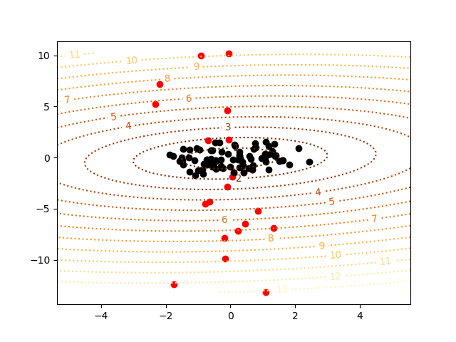
(4) 点模式分析的离群值发现( MinCovDet - Minimum Covariance Determinant (MCD))
SCIKIT-LEARN中,非高斯分布可采用 OneClassSVM; 高斯分布数据可采用 MinCovDet和 EmpiricalCovariance,效果较好。其中, MinCovDet 鲁棒性好于 EmpiricalCovariance( 最大似然估计, MLE)。 二者都是用来估计出样本集的中心和形状参数,用于决定一个同样本集拟合程度最好的一个理论密度分布曲面。
EmpiricalCovariance( 经验协方差估计, 采用样本的最大似然估计法 MLE),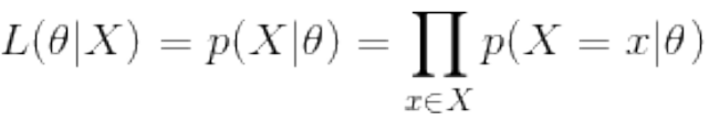 , 就是要用似然函数取到最大值时的参数值作为估计值。 为何要使 L 最大呢,因为 X 已经发生了( 基于某一个参数发生的), 通常它是属于那种最大概率的情况。通
常, EmpiricalCovariance 受噪声影响比较大。
MinCovDet( 最小协方差决定因子算法?),适用于高斯分布数据,也可以用于单峰分布的数据(多峰不可以!)。 可以处理至多含有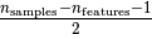 离群值的样本集, 主要思想是寻找
 个样本,使得协方差矩阵 determinant 行列式值最小。
确定离群值: 针对一个多维正态分布( 假设为高斯分布, 如: 2 维),其分布曲面是一个密度曲面。一个样本点到该分布中心的马氏距离( Mahalanobis), 其数值大小决定了该点
是否离群值。
以下代码是用理论分布1生成黑点,用理论分布2生成红点(较少),希望估算的时候基于黑点估算出它的分布,排除红点噪音。
 1 import numpy as np
 2 import matplotlib.pyplot as plt
 3
 4 from sklearn.covariance import EmpiricalCovariance, MinCovDet
 5
 6 n_samples = 125
 7 n_outliers = 25
 8 n_features = 2
 9
10 # generate data
11 gen_cov = np.eye(n_features)
12 gen_cov[0, 0] = 2.#主对角线00位置上赋值为2
13 #生成了125个属性点,每个点有2个属性,后面又乘了2行2列的主矩阵
14 X = np.dot(np.random.randn(n_samples, n_features), gen_cov)
15 # add some outliers
16 outliers_cov = np.eye(n_features)
17 #生成了1个1,相当于将(1,1)位置上换成了7
18 outliers_cov[np.arange(1, n_features), np.arange(1, n_features)] = 7.
19 #将倒数的25个样本给换了,从-多少开始,往下数,省略了一个冒号
20 X[-n_outliers:] = np.dot(np.random.randn(n_outliers, n_features), outliers_cov)
21
22 #参数估计
23 # fit a Minimum Covariance Determinant (MCD) robust estimator to data
24 #MinCovDet()相当于调构造函数
25 robust_cov = MinCovDet().fit(X)
26
27 #全样本得到n个马氏距离,给评价函数,迭代
28 # compare estimators learnt from the full data set with true parameters
29 emp_cov = EmpiricalCovariance().fit(X)
30
31 #打一个q就退出来了
32
33 #结果
34 # Estimated robust location (n_features,), 均值
35 robust_cov.location_
36 #array([-0.00320609, -0.07327767])
37
38
39 # Estimated robust covariance matrix (n_features, n_features),协方差矩阵
40 robust_cov.covariance_
41 #array([[2.25467783, 0.22281682],
42 #       [0.22281682, 1.03483927]])
43
44
45 #规则网格 100x100, numpy.ravel - return a contiguous flattened array
46 xmin,ymin = list(np.min(X,axis=0))#打格子,样本值的第一列
47 xmax,ymax = list(np.max(X,axis=0))
48 #xx.ravel().shape 维数1维,里面含有10000个数
49 xx, yy = np.meshgrid(np.linspace(xmin,xmax, 100), np.linspace(ymin,ymax, 100))
50 xy = np.concatenate([xx.ravel()[:,np.newaxis], yy.ravel()[:,np.newaxis]], axis=1)
51
52 #马氏距离表示点与一个分布之间的距离。 对于一个均值为 μ, 协方差矩阵为 Σ 的多变量
53 #向量,其马氏距离为 sqrt( (x-μ)'Σ^(-1)(x-μ) )
54 mahal_robust = robust_cov.mahalanobis(xy) #表示数据的协方差距离
55 mahal_robust = mahal_robust.reshape(xx.shape)
56
57 #mahal_emp = emp_cov.mahalanobis(xy)
58 #mahal_emp = mahal_emp.reshape(xx.shape)
59
60 mahal_X = robust_cov.mahalanobis(X)
61 X_ = X[np.where(mahal_X<=3)] #信号数据 mahal马氏距离,
62 X__ = X[np.where(mahal_X>3)] #噪音数据
63
64 ###############################################################################
65 # Display results
66 fig = plt.figure()#定义figure,相当于一张纸
67 #plt.scatter(X[:, 0], X[:, 1], color='black', label='inliers')
68 #从倒数第25个取,倒数125个值
69 plt.scatter(X[:, 0][-n_outliers:], X[:, 1][-n_outliers:], color='red', label='outliers')
70 plt.scatter(X_[:, 0], X_[:, 1], color='black', label='selected')
71 levels = np.arange(1, 16, 1)
72 #等高线
73 robust_cs = plt.contour(xx, yy, np.sqrt(mahal_robust),levels=levels, cmap=plt.cm.YlOrBr_r,linestyles='dotted')
74 plt.clabel(robust_cs, inline=1, fmt='%d', fontsize=10)
75 #emp_cs = plt.contour(xx, yy, np.sqrt(mahal_emp), cmap=plt.cm.YlOrBr_r, linestyles='dotted')
76 #plt.clabel(emp_cs, inline=1, fmt='%d', fontsize=10)
77 plt.show()
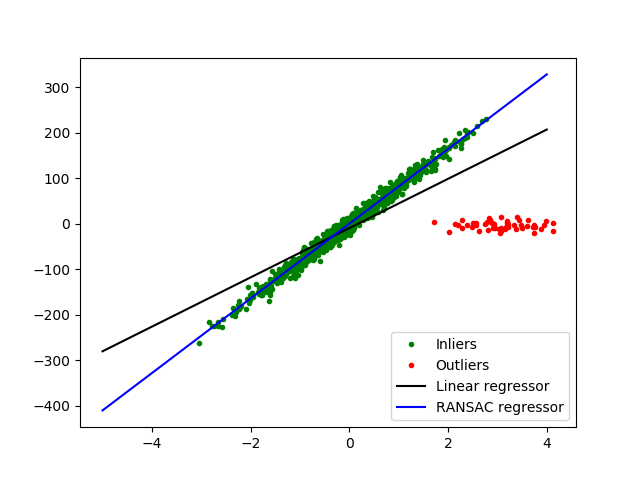
(5) RANSAC (RANdom SAmple Consensus)
RANSAC 是一个迭代模型,通过从包含噪音观测样本中随机取样,估计纯样本(信号) 的理论分布模型。
主要分为两大步骤:
1)首选选择一个样本子集,数目必须满足一个基数,估算出模型参数。
2)然后检查整个数据集的样本是否和该模型一致,给定一个阈值或评估函数,偏离该模型的样本为离群值,符合者构成一个新样本集。
重复上述两个步骤,直到获得一个含有足够多样本的数据子集(有效数据)。其中, 步骤( 2)可能获得一个样本很少的子集,模型被拒绝;也可能获得一个样本多的子集,模型参数可以
被进一步细化。
RANSAC 中用于建模的分布模型,必须具有 fit(X, y), score(X, y)两个函数。 前者用样本拟合模型,后者返回样本数据精度,以便判断是否结束迭代。
例如: 拟合线性模型,剔除离群值
 1 #RANSAC
 2 #避开异常点做迭代回归,参数估计,正向评价
 3
 4 """
 5 ===========================================
 6 Robust linear model estimation using RANSAC
 7 ===========================================
 8 """
 9 import numpy as np
10 from matplotlib import pyplot as plt
11 from sklearn import linear_model, datasets
12
13 n_samples = 1000
14 n_outliers = 50
15
16 #生成1000个样本,feature只有1个,噪音含10个
17 X, y, coef = datasets.make_regression(n_samples=n_samples, n_features=1, \
18                                       n_informative=1, noise=10, \
19                                       coef=True, random_state=0)
20
21 # Add outlier data
22 np.random.seed(0)
23 #生成50个样本,放在1000个样本前面
24 X[:n_outliers] = 3 + 0.5 * np.random.normal(size=(n_outliers, 1))
25 y[:n_outliers] = -3 + 10 * np.random.normal(size=n_outliers)
26
27 # Fit line using all data
28 model = linear_model.LinearRegression()
29 model.fit(X, y)
30
31 # Robustly fit linear model with RANSAC algorithm
32 #RANSAC迭代的每一个步骤还是线性回归
33 #估算还是靠的linear_model
34 #inlier,outlier信号,噪音
35 #mask,把true的取出来
36 model_ransac =linear_model.RANSACRegressor(base_estimator=linear_model.LinearRegression())
37 model_ransac.fit(X, y)
38 inlier_mask = model_ransac.inlier_mask_
39 outlier_mask = np.logical_not(inlier_mask)#取反,就是噪音
40
41 # Predict data of estimated models
42 line_X = np.arange(-5, 5)#生成了10个x值,等间隔为1
43 line_y = model.predict(line_X[:, np.newaxis])#预测出它的y值出来,画出黑色的直线
44 line_y_ransac = model_ransac.predict(line_X[:, np.newaxis])
45 print ('y = ax +b, a=? b=?')
46 #将RANSAC估计的a,b值打出来
47 print (model_ransac.estimator_.coef_, model_ransac.estimator_.intercept_)
48
49 # Compare estimated coefficients
50 print ("Estimated coefficients (true, normal, RANSAC):")
51 print (coef, model.coef_, model_ransac.estimator_.coef_)
52
53 plt.plot(X[inlier_mask], y[inlier_mask], '.g', label='Inliers')
54 plt.plot(X[outlier_mask], y[outlier_mask], '.r', label='Outliers')
55 plt.plot(line_X, line_y, '-k', label='Linear regressor')
56 plt.plot(line_X, line_y_ransac, '-b', label='RANSAC regressor')
57 plt.legend(loc='lower right')
58 plt.show()
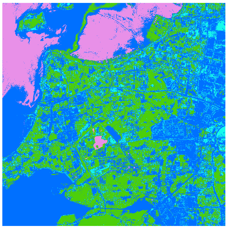
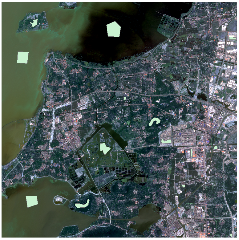
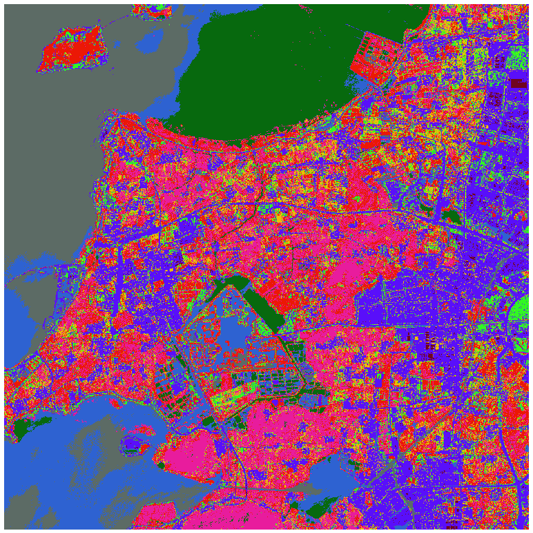
2. 分类问题( 一个遥感图像分类的例子 – 贝叶斯分类器,决策树,知识向量机等)
分类是机器学习的一大类问题。解决分类需要理解( 1) 数据预处理、( 2) 特征提取、( 3)分类方法、以及( 4) 结果评估等关键环节。
#数据预处理
数据的标准化(Standardization)/归一化(Normalization), 具体定义?
将数据按比例缩放,使之落入一个小的特定区间。在某些比较和评价的指标处理中经常会用到,去除数据的单位限制,将其转化为无量纲的纯数值,便于不同单位或量级的指标能够进行比较和加权。 主要目的:
1 把数变为特定区间的数值, 如: [0,1]内的小数为了数据处理方便提出来的,把数据映射到特定范围之内, 提高处理便捷性。
2 把有量纲表达式变为无量纲表达式
简化计算方式, 将有量纲的表达式, 变换为无量纲的表达式,成为纯量。
常见方法:
(1) min-max 标准化(Min-max standardization) --->[0,1]
(x-min)/(max-min)
(2) z-score 标准化(zero-mean normalization),
(x-mean)/std
(3) log 函数转换
(4)atan 函数转换
用反正切函数也可以实现数据的归一化。
… …
#通常,机器学习算法中的梯度方法对于数据的缩放和尺度都是很敏感的, scikit-learn 预处理使得特征数据缩放到 0-1 范围中
https://www.cnblogs.com/pejsidney/p/8031250.html
实际上下面这段代码几乎都不懂
  1 #通常,机器学习算法中的梯度方法对于数据的缩放和尺度都是很敏感的, scikit-learn 预处
  2 理使得特征数据缩放到 0-1 范围中
  3 #https://www.cnblogs.com/pejsidney/p/8031250.htm
  4 #
  5 from sklearn import preprocessing
  6
  7 #scale, (X - X_mean)/X_std #standard scaler对数据做归一化的公式
  8 x = np.arange(9).reshape(3,3)#原始数据,3行3列
  9 scaler = preprocessing.StandardScaler()
 10 scaler.fit(x) #算scaler归一化的参数
 11 x_scale = scaler.transform(x)#将x集合里的每一个样本减均值除以标准差
 12 np.min(x_scale), np.max(x_scale), np.mean(x_scale), np.std(x_scale)
 13 #
 14 x
 15
 16 #scale, X_std=(X - min)/(max-min)做拉伸
 17 x = np.arange(9).reshape(3,3)
 18 scaler = preprocessing.MinMaxScaler()
 19 scaler.fit(x)
 20 x_scale = scaler.transform(x)
 21 np.min(x_scale), np.max(x_scale), np.mean(x_scale), np.std(x_scale)
 22
 23
 24 #binarize二值化,给阈值,0,1
 25 x = np.arange(9).reshape(3,3)
 26 binarizer = preprocessing.Binarizer(threshold= 4)
 27 x_bin = binarizer.transform(x)
 28 np.min(x_bin), np.max(x_bin), np.mean(x_bin), np.std(x_bin)
 29 #
 30 x_bin
 31
 32 #normalize #第一个是按列来算的,后面的是按所有的来算的
 33 x = np.arange(9).reshape(3,3)
 34 norm = preprocessing.Normalizer()
 35 norm.fit(x)
 36 x_norm = norm.transform(x)
 37 np.min(x_norm), np.max(x_norm), np.mean(x_norm), np.std(x_norm)
 38
 39 #遥感图像读取与分类
 40 #
 41 import numpy as np
 42 import sys
 43 sys.path.append( r'E:\选课复习\研一上\Python\week7\chapter_06' )
 44 from gwp_image import IMAGE
 45
 46 #图像和训练区读取
 47 drv = IMAGE()
 48 im_proj,im_geotrans,im_data = drv.read_img('taihu_gf2.tif')
 49 ao_proj,ao_geotrans,ao_data = drv.read_img('taihu_gf2_aoi.tif')
 50 band,row,col = im_data.shape
 51
 52 im_data = np.swapaxes(np.swapaxes(im_data,0,1),1,2)#0轴1轴交换,维数变为2400,2000,第一次交换的结果1,2又做一次交换
 53 print (im_data.shape, ao_data.shape)
 54 #(2000, 2000, 4) (2000, 2000)
 55
 56 #
 57 im_data[0,0]
 58 #array([442, 380, 215,  74], dtype=uint16)
 59
 60 #reshape into m_sample*n_feaure
 61 im_data = im_data.reshape(row*col, band)
 62 ao_data = ao_data.reshape(row*col)
 63 print (im_data.shape, ao_data.shape)
 64 #(4000000,4)(4000000,)
 65
 66 im_data.shape
 67 #(4000000, 4)
 68
 69 #im_data[0,:]
 70 #array([442, 380, 215,  74], dtype=uint16)#变换的结果要对
 71
 72 ao_data.shape
 73 #(4000000,)
 74
 75 np.uint(ao_data)
 76
 77 #样本数据
 78 from sklearn import preprocessing
 79 from sklearn.model_selection import KFold
 80
 81 #sampling data
 82 x_sample = im_data[np.where(ao_data>0)]#ao_data像元属于哪一个类
 83 y_sample = ao_data[np.where(ao_data>0)]
 84
 85 samples = np.concatenate([x_sample, y_sample [:,np.newaxis]],axis=1)#沿着列合,沿着1轴
 86 #samples.shape
 87 #samples[0,:]
 88 #像元的波段值,属于哪一类
 89
 90 # n_splits=3, 2/3 training, 1/3 verfying, 交叉验证 3 次
 91 k_fold = KFold(n_splits=3, shuffle=False) #shuffle=True, 随机数种子启用, 则每次分组不同
 92 cp=0
 93 for train, test in k_fold.split(samples):
 94     #print('Train: %s | test: %s' % (train_indices, test_indices))
 95     cp+=1
 96     print (samples[ train].shape, samples[test].shape)
 97
 98 #train set
 99 x_train = samples [train][:,:-1]
100 y_train = samples [train][:,-1]
101
102 #test set
103 x_test = samples [test][:,:-1]
104 y_test = samples [test][:,-1]
105
106 #特征选择(Feature Selection)
107 '''
108 样本具有多个特征(或属性),对于分类或回归等建模问题,这些特征起到了不同的作用,
109 有的相关性强则贡献大些,而有的则比较弱。特征选择是困难的,经验和专业知识很重要,
110 但是 scikt-learn 有现成的算法支持特征选择。
111 '''
112 #树算法(Tree algorithms)是用于计算特征的信息量的一种常见方法
113 #
114 from sklearn import metrics
115 from sklearn.ensemble import ExtraTreesClassifier
116 model = ExtraTreesClassifier()
117
118 scaler = preprocessing.StandardScaler ()
119 scaler.fit(x_train)
120 x_train = scaler.transform(x_train)#原始数据0~255个值来训练结果
121 x_test = scaler.transform(x_test)
122
123 model.fit(x_train, y_train)
124 print(model.feature_importances_)
125 #[0.30527885 0.32615108 0.18510445 0.18346563]
126
127 #朴素贝叶斯
128 #著名的机器学习算法,还原训练样本数据的分布密度,其在多类别分类中有很好的效果
129 #最大似然分类是朴素贝叶斯分类的特例,假设各类别的先验概率相等。
130 from sklearn import metrics
131 from sklearn.naive_bayes import GaussianNB#高斯分类器
132 model = GaussianNB()
133
134 model.fit(x_train, y_train)
135
136 y_pred = model.predict(x_train)#预测
137 len(np.where((y_pred-y_train)==0)[0])
138 #33153
139 y_pred = model.predict(x_test)
140 len(np.where((y_pred-y_test)==0)[0])#3365应该接近y_test.shape
141 #3365
142 #y_test.shape
143 #(16947,)实际上并不接近
144
145 #
146 im_labe = model.predict( scaler.transform(im_data) )#把原始数据全部做一遍分类
147 #im_data[0,]
148 #array([442,380,215,74])看一看im_data是说明数据
149 im_labe = im_labe.reshape(row,col)
150 print (np.unique(np.array(im_labe), return_counts=True) ) #??
151 im_labe = ((im_labe/10).astype(np.uint8))*10#将2000行2000列里的数据都除以10,按大类来,10,20,30
152
153 drv.write_img('taihu_gf2_lab01.tif',im_proj,im_geotrans,im_labe)#分类效果感觉并不好
154
155 #np.unique(im_labe)
156 #array([10,20,30,40])
157
158 #2/4=0.5 3.0以后算出小数来了,和过去不一样
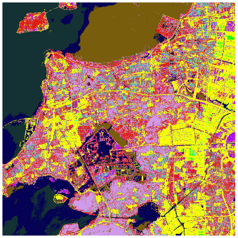
#决策树
#分类与回归树(Classification and Regression Trees ,CART)算法常用于特征含有类别信息的分类或者回归问题,适用于多分类情况
#计算每类在一个属性上的信息熵,根据信息熵之间的差异,选定信息熵最大的属性最为最好的分类依据先进行分类。
唯一不同是构造函数不同,fit训练模型,predict用训练好的模型对整幅图像进行预测。
 1 from sklearn import metrics
 2 from sklearn.tree import DecisionTreeClassifier
 3 model = DecisionTreeClassifier()
 4 model.fit(x_train, y_train)
 5 y_pred = model.predict(x_train)
 6 len(np.where((y_pred-y_train)==0)[0])
 7 #33896
 8 y_pred = model.predict(x_test)
 9 len(np.where((y_pred-y_test)==0)[0])
10 #3388
11 #
12 im_labe = model.predict( scaler.transform(im_data) )
13 im_labe = im_labe.reshape(row,col)
14 print (np.unique(np.array(im_labe), return_counts=True) ) #
15 im_labe = (im_labe/10)*10
16
17 drv.write_img('taihu_gf2_lab02.tif',im_proj,im_geotrans,im_labe)
#支持向量机
#SVM 是非常流行的机器学习算法,主要用于分类问题,适用于一对多或多分类
 1 #
 2 from sklearn import metrics
 3 from sklearn.svm import SVC
 4
 5 model.fit(x_train, y_train)
 6
 7 y_pred = model.predict(x_train)
 8 len(np.where((y_pred-y_train)==0)[0])
 9 #33896
10 y_pred = model.predict(x_test)
11 len(np.where((y_pred-y_test)==0)[0])
12 #3388
13 #
14 im_labe = model.predict( scaler.transform(im_data) )
15 im_labe = im_labe.reshape(row,col)
16 print (np.unique(np.array(im_labe), return_counts=True) ) #
17 im_labe = (im_labe/10)*10
18
19 drv.write_img('taihu_gf2_lab03.tif',im_proj,im_geotrans,im_labe)
#结果评估或模型选择,针对三个模型依次执行,查看混淆矩阵的结果
 1 print(model)
 2 '''
 3 DecisionTreeClassifier(class_weight=None, criterion='gini', max_depth=None,
 4                        max_features=None, max_leaf_nodes=None,
 5                        min_impurity_decrease=0.0, min_impurity_split=None,
 6                        min_samples_leaf=1, min_samples_split=2,
 7                        min_weight_fraction_leaf=0.0, presort=False,
 8                        random_state=None, splitter='best')
 9
10 '''
11 # make predictions
12 measured = y_test
13 predicted = model.predict(x_test)
14 # summarize the fit of the model
15 print(metrics.classification_report(measured, predicted))
16 #非常低,只有0.2,...都是3000多
17 print(metrics.confusion_matrix(measured, predicted))
18
19 #50000多个样本,Kfold分成两部分,给成false,关闭了采样的随机性,导致可能一些样本都没有
3.再论回归问题, 网格搜索与交叉验证的用途
给定一组样本(含因变量值和自变量值),数学建模时模型参数的求解是一个关键问题。模型参数分两大类:一类是利用样本数据,通过数学模型反演和机器学习可以获得的参数,一类是凭借经验值或者统计与数据集特征相关的参数。
网格搜索(随机搜索) 与交叉验证主要用于在一个给定的参数分布空间内,搜索那些数学模型不能通过机器学习估算的参数,通过交叉验证,选出得分最高的参数作为模型最优输入。
例如:知识向量机的罚函数 C 与 gamma ( RBF), Ridge 模型的 alpha 参数, Lasso 模型的 alpha参数等。
网格搜索 – 类似穷举法, 获得每个枚举参数组合的模型误差, 使得模型误差最小的参数对为优化解。 但是可以通过粗网格初选和细网格精选提高参数搜索效率;随机搜索 – 参数符合一个数学分布,多个参数搜索仍能保持较高搜索效率。
(1) 以一个房屋价格回归模型为例。
https://archive.ics.uci.edu/ml/datasets.html
https://archive.ics.uci.edu/ml/machine-learning-databases/housing/housing.names
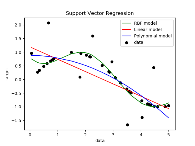
  1 #3.再论回归问题,网格搜索与交叉验证的用途
  2
  3 #数据读取
  4 import numpy as np
  5 fh= open("housing.data")
  6 #506行的大字符串
  7 #对这一行先去了首尾的空白字符,包括空格,table,回车键\n,unix的\f
  8 #成了506行,14列
  9 raw_data = [[float(v) for v in ln.strip().split()] for ln in fh.readlines()]
 10 fh.close()
 11 #强制转为32位,减少内存占用
 12 dataset = np.array(raw_data).astype(np.float32)
 13 #要了13行以前的,第14行是价格
 14 X = dataset[:,0:13]
 15 y = dataset[:,13]
 16
 17 #多元回归+惩罚函数
 18 import numpy as np
 19 from sklearn.linear_model import Ridge#类名,惩罚函数的系数,只能是咱们给
 20 #from sklearn.grid_search import GridSearchCV 由于版本问题,这一句不能执行
 21 from  sklearn.model_selection import GridSearchCV
 22 # prepare a range of alpha values to test
 23 alphas = np.array([1,0.1,0.01,0.001,0.0001,0])
 24 alphas = np.array([0.01,0.001,0.0001,0])
 25 # create and fit a ridge regression model, testing each alpha
 26 model = Ridge(fit_intercept=True, solver='svd')#ridge回归模型初始化,每个自变量前面加个待定系数,后边再加个Bata
 27 # solver : {'auto', 'svd', 'cholesky', 'lsqr', 'sparse_cg', 'sag'}#多种办法帮助求出待定系数的w
 28 #给定α的情况下求待定系数cv,用ridge模型做回归,α用刚才给的那个数,param_grid是写死的
 29 #若是以简单参数必填的,直接给参数值,否则就用dict的格式
 30 #出的结果都会放在grid里
 31 grid = GridSearchCV(estimator=model, param_grid=dict(alpha=alphas))
 32 grid.fit(X, y)
 33 print(grid)
 34 '''
 35 GridSearchCV(cv='warn', error_score='raise-deprecating',
 36              estimator=Ridge(alpha=1.0, copy_X=True, fit_intercept=True,
 37                              max_iter=None, normalize=False, random_state=None,
 38                              solver='svd', tol=0.001),
 39              iid='warn', n_jobs=None,
 40              param_grid={'alpha': array([0.01  , 0.001 , 0.0001, 0.    ])},
 41              pre_dispatch='2*n_jobs', refit=True, return_train_score=False,
 42              scoring=None, verbose=0)
 43
 44 '''
 45
 46 # summarize the results of the grid search
 47 print(grid.best_score_)
 48 #-1.5507356822683775
 49 print(grid.best_estimator_.alpha) #alpha
 50 #0.01
 51 print(grid.best_estimator_.coef_) #斜率
 52 '''
 53 [-1.0795517e-01  4.6437558e-02  2.0076692e-02  2.6850116e+00
 54  -1.7652218e+01  3.8107793e+00  5.9260055e-04 -1.4738853e+00
 55   3.0578226e-01 -1.2343894e-02 -9.5147777e-01  9.3177296e-03
 56  -5.2488232e-01]
 57
 58 '''
 59 print(grid.best_estimator_.intercept_) #截距
 60 #36.378204
 61
 62 #给个新区间,多级网格搜索
 63
 64 #平均误差 STD,平均房价( 1000$)
 65 #delta是预测价格和实际价格的差异
 66 delta = np.dot(X,grid.best_estimator_.coef_) + grid.best_estimator_.intercept_ - y
 67 #求平方取均值开方
 68 print(np.sqrt(np.mean(np.square(delta))), np.mean(y))
 69 #4.6791954 22.532806
 70
 71 #特征选取, SelectFromModel, #from version 0.17
 72 #13个变量,想挑出其中特别重要的
 73 from sklearn.feature_selection import SelectFromModel
 74 model = SelectFromModel(grid.best_estimator_, prefit=True)
 75 X_new = model.transform(X)
 76 X_new.shape
 77 #(506, 3)
 78 X.shape
 79 #(506, 13)
 80
 81 X_new[2,:]
 82 #从13列里挑出了3列
 83
 84 #支持向量机回归(知识向量机?)
 85
 86 # #
 87 #Grid-search and Cross-validated estimators
 88 #These estimators are called similarly to their counterparts, with ‘CV’ appended to their name
 89
 90 from  sklearn.model_selection import GridSearchCV
 91 from sklearn.model_selection import KFold, cross_val_score
 92 from sklearn.svm import SVR
 93 import numpy as np
 94 import matplotlib.pyplot as plt
 95
 96 ###############################################################################
 97 # Generate sample data
 98 X = np.sort(5 * np.random.rand(40, 1), axis=0) #40个随机数,乘以5,0-5之间
 99 y = np.sin(X).ravel()#求了sin值
100
101 ###############################################################################
102 # Add noise to targets
103 y[::5] += 3 * (0.5 - np.random.rand(8)) #间隔 5,取数据,0.5减去8个随机数,
104 #范围在-1.5 - +1.5原来样本里的8个数据,加了噪音
105 #40个数每隔5个数取出来,取了8个数出来
106 y
107 y[::5]
108
109 ###############################################################################
110 # Fit regression model
111 svr_rbf = SVR(kernel='rbf', C=1e3, gamma=0.1)
112 svr_lin = SVR(kernel='linear', C=1e3)#线性函数作为支持向量机的核函数
113 svr_poly = SVR(kernel='poly', C=1e3, degree=2)
114 y_rbf = svr_rbf.fit(X, y).predict(X)
115 y_lin = svr_lin.fit(X, y).predict(X)
116 y_poly = svr_poly.fit(X, y).predict(X)
117 ###############################################################################
118 # look at the results
119 plt.scatter(X, y, c='k', label='data')
120 plt.hold('on') #保持当前绘图和所有轴属性(包括当前颜色和线型),以便随后绘图命令不重#
121 #上一句代码有点问题,会报错,无法执行
122 #AttributeError: module 'matplotlib.pyplot' has no attribute 'hold'
123 #置颜色和线型; off 返回默认模式, PLOT 命令借此擦出前面的绘图并重置新图所有坐标属
124 性。
125 plt.plot(X, y_rbf, c='g', label='RBF model')
126 plt.plot(X, y_lin, c='r', label='Linear model')
127 plt.plot(X, y_poly, c='b', label='Polynomial model')
128 plt.xlabel('data')
129 plt.ylabel('target')
130 plt.title('Support Vector Regression')
131 plt.legend()
132 plt.show()
133 ###############################################################################
134 # grid search of svm for perfect parameters
135 C = np.array([2000,1000,500,250,125])
136 g = np.array([1,0.5,0.25,0.125])
137 svr_rbf = SVR(kernel='rbf')
138 grid = GridSearchCV( estimator= svr_rbf, param_grid=dict(C=C,gamma=g) )#给区间网格搜索
139 grid.fit(X, y)
140 print(grid)
141 '''
142 GridSearchCV(cv='warn', error_score='raise-deprecating',
143              estimator=SVR(C=1.0, cache_size=200, coef0=0.0, degree=3,
144                            epsilon=0.1, gamma='auto_deprecated', kernel='rbf',
145                            max_iter=-1, shrinking=True, tol=0.001,
146                            verbose=False),
147              iid='warn', n_jobs=None,
148              param_grid={'C': array([2000, 1000,  500,  250,  125]),
149                          'gamma': array([1.   , 0.5  , 0.25 , 0.125])},
150              pre_dispatch='2*n_jobs', refit=True, return_train_score=False,
151              scoring=None, verbose=0)
152
153 '''
154 print(grid.best_estimator_)
155 '''
156 SVR(C=500, cache_size=200, coef0=0.0, degree=3, epsilon=0.1, gamma=0.25,
157     kernel='rbf', max_iter=-1, shrinking=True, tol=0.001, verbose=False)
158
159 '''
4.聚类分析
4.1 Scikt-learn支持的聚类方法
http://scikit-learn.org/stable/modules/clustering.html#clustering
常见聚类方法的 API 调用方法:
不同的聚类方法需要输入参数不同,如:类别数目、阈值、每类最少样本数等。有的自动化程度高些,有的需要用户不断测试参数直到获得一个较好质量的结果。
下面这部分代码能够跑一遍,但是对于具体的意义并没有理解。
  1 #4 聚类分析
  2 #4.1 Scikit-learn支持的聚类方法
  3 #让稀疏地方的点向密集地方的点位移,第二圈再迭代,重新计算密度,所有点都向最大密度地方做位移
  4 #无限循环下会形成几个聚类中心
  5 #最后一点点位移到聚类中心
  6 #迭代过程每一步样本点所有移的位置串成一根线,像河流形成聚类中心
  7 #生成样本
  8 #属性加距离形成权重
  9 import numpy as np
 10 from sklearn.datasets.samples_generator import make_blobs
 11 # we create separable points
 12 X, Y = make_blobs(n_samples=100, centers=2, random_state=0, cluster_std=0.60)
 13 X, Y = make_blobs(n_samples=1500, cluster_std=[1.0, 2.5, 0.5], random_state=170)#3个聚类中心
 14 X.shape
 15 #(1500,2)
 16 Y.shape
 17 #(1500,)
 18 #Y代表在坐标上面会有属性值
 19
 20
 21 # 聚类 – MeanShift
 22 cluster_name = "MeanShift"
 23 from sklearn.cluster import MeanShift, estimate_bandwidth
 24 #ms = MeanShift(bandwidth=estimate_bandwidth(X, quantile=0.2, n_samples=1500), bin_seeding=True)
 25 #带宽指针对某一列的值求标准差,相当于求波动范围
 26 ms = MeanShift(bandwidth=estimate_bandwidth(X, n_samples=1500), bin_seeding=True)
 27 #fit函数放进去
 28 ms.fit(X)
 29 #ms.labels_分了若干个类
 30 labels = ms.labels_
 31 #np.unique(labels)
 32 #array([0, 1, 2], dtype=int64),0是未分类的,1是一类,2是一类
 33 #1500个点,分两簇
 34 cluster_centers = ms.cluster_centers_
 35 cluster_centers.shape
 36 #(3,2)每个样本有两个属性
 37 cluster_centers
 38 '''
 39 array([[ 1.85568743,  0.44433028],
 40        [-8.92178147, -5.45806097],
 41        [-4.68205739, -0.28572227]])
 42
 43 '''
 44 labels.shape
 45 #(1500,)
 46 X.shape
 47 #(1500,2)
 48 np.where(labels==1)
 49 #打算取数据
 50 X[np.where(labels==2),:].shape
 51 #(1,423,2)多了1,有错误,拿出了432行不是一个数组,而是数组外又套了个数组,应该要的是行的下标
 52 X[np.where(labels==2)].shape
 53 #(423, 2)
 54 X[np.where(labels==2)[0],:].shape#结果同上
 55 Y.shape
 56 #(1500,)
 57 np.unique(Y)
 58 #array([0,1,2])
 59 Y[np.where(labels==2)[0]].shape
 60 #(423,)
 61 #预测出的0有可能对应Y里的2
 62
 63 n_clusters_ = len(np.unique(labels))
 64 print("number of estimated clusters : %d" % n_clusters_)
 65 #number of estimated clusters : 3
 66
 67
 68 # 聚类 – DBSCAN
 69 '''
 70 ( 参数: 半径 eps, MinPts;关键词: 邻居、 核心点/边缘点/离群点、 密度(直接) 可达, 密度(直接)
 71 可达的若干核心对象及其邻域内的边缘点形成一个聚类簇)
 72 '''
 73
 74 cluster_name = " DBSCAN"
 75 from sklearn.cluster import DBSCAN
 76 #eps : The maximum distance between two samples for them to be considered as in the sameneighborhood.
 77 #min_samples : The number of samples (or total weight) in a neighborhood for a point to be
 78 #considered as a core point. This includes the point itself.
 79 #
 80 ms= DBSCAN (eps=0.75,min_samples=10)#eps找邻居找半径,看密度
 81 ms.fit (X)
 82 '''
 83 DBSCAN(algorithm='auto', eps=0.75, leaf_size=30, metric='euclidean',
 84        metric_params=None, min_samples=10, n_jobs=None, p=None)
 85
 86 '''
 87 labels = ms.labels_
 88 #cluster_centers = ms.cluster_centers_
 89 n_clusters_ = len(np.unique(labels))
 90 print("number of estimated clusters : %d" % n_clusters_)
 91 #number of estimated clusters : 5
 92
 93 # 聚类 - KMeans#M类给了M个初始化的中心,每一轮迭代都对聚类中心有一定的校正,当聚类中心
 94 #不再偏移
 95 cluster_name = "KMeans"
 96 from sklearn.cluster import KMeans
 97 ms=KMeans(n_clusters=3, random_state=170)
 98 ms.fit(X)
 99 labels = ms.labels_
100 cluster_centers = ms.cluster_centers_
101 n_clusters_ = len(np.unique(labels))
102 print("number of estimated clusters : %d" % n_clusters_)
103 #number of estimated clusters : 3
104
105 # 聚类 – AgglomerativeClustering (Hierarchical clustering 层次聚类)
106 #层次聚类能够不用给定分多少类,可以给定阈值自动决定类数
107 #n个样本,有n个类,每个样本聚类中心就是样本所在的位置
108 #任何两个点之间算距离,算最短距离,挑邻居合成一类,n类->n-1类
109 #新的聚类中心,两个加起来求平均
110 #3,4个点有12中连接方式
111 cluster_name = " AgglomerativeClustering "
112 from sklearn.cluster import AgglomerativeClustering
113 #用于层次聚类的“ 距离” 定义, 用于判断是否合并
114 #complete - 元素对之间的最大距离
115 #single - 元素对之间的最小距离
116 #group average – 组间样本距离的平均值
117 #ward – “距离”指两簇 ESS 的和, 同合并后新簇 ESS 的差值( 增量), ESS=Σ(xi-x_mean)**2
118 ms= AgglomerativeClustering (linkage="ward", n_clusters=3) #'ward', 'average', 'complete'
119 ms.fit(X)
120 '''
121 AgglomerativeClustering(affinity='euclidean', compute_full_tree='auto',
122                         connectivity=None, distance_threshold=None,
123                         linkage='ward', memory=None, n_clusters=3,
124                         pooling_func='deprecated')
125 '''
126 labels = ms.labels_
127 #cluster_centers = ms.cluster_centers_
128 n_clusters_ = len(np.unique(labels))
129 print("number of estimated clusters : %d" % n_clusters_)
130 '''
131 number of estimated clusters : 3
132 '''
133 # 聚类 - spectral_clustering
134 # #谱聚类
135 #从图像分割来的
136 #将每一个像元看成一个点,每个点上有一组属性值
137 #任何一个像元都与周围像元连了8根线,任何一个点能到达任一个点
138 #连线需要计算权重,直线连接,对角线连接,波谱值相近程度,波谱值接近
139 # 这两个点属于同一类,找出权限最弱的那一个打断,最后形成孤岛
140 #
141 cluster_name = " spectral_clustering"
142 from sklearn.neighbors import kneighbors_graph
143 from sklearn.cluster import spectral_clustering
144
145 #没法标准化,计算速度慢,前面fit一下就可以,这里不行,它会把样本转为一个图
146 graph = kneighbors_graph(X, 25)
147 labels= spectral_clustering(graph, n_clusters=3, eigen_solver='arpack')
148 n_clusters_ = len(np.unique(labels))
149 print("number of estimated clusters : %d" % n_clusters_)
150 #number of estimated clusters : 3
151
152 #绘图显示聚类结果
153 import matplotlib.pyplot as plt
154 X0 = X[np.where(labels==0)]
155 X1 = X[np.where(labels==1)]
156 X2 = X[np.where(labels==2)]
157 plt.plot(X[:,0],X[:,1],'ko')
158 plt.plot(X0[:,0],X0[:,1],'ro')
159 plt.plot(X1[:,0],X1[:,1],'bo')
160 plt.plot(X2[:,0],X2[:,1],'go')
161 plt.title(cluster_name)
162 plt.show()
163
164 #4.2非常非常慢,图像分割会分成非常少,50x50个,2000个像素的样本