


4.Ceres官方教程-非线性最小二乘~Curve Fitting(曲线拟合)
1.Curve Fitting
到目前为止,我们看到的示例都是没有数据的简单优化问题。最小二乘和非线性最小二乘分析的原始目的是对数据进行曲线拟合。
接下来将介绍曲线拟合的问题。采样点是根据曲线 生成的,并且添加标准差σ=0.2的高斯噪声。我们用下列带未知参数的方程来拟合这些采样点:

首先定义一个模板对象来计算残差。每一个观察值(采样点)都有一个残差。
struct ExponentialResidual {
  ExponentialResidual(double x, double y)
      : x_(x), y_(y) {}

  template <typename T>
  bool operator()(const T* const m, const T* const c, T* residual) const {
    residual[0] = y_ - exp(m[0] * x_ + c[0]);
    return true;
  }

 private:
  // Observations for a sample.
  const double x_;
  const double y_;
};
假设观测数据是一个名为data的2n大小的的数组,为每一个观察值创建一个CostFunction的问题(problem)构造是一个简单的事。
double m = 0.0;
double c = 0.0;

Problem problem;
for (int i = 0; i < kNumObservations; ++i) {
  CostFunction* cost_function =
       new AutoDiffCostFunction<ExponentialResidual, 1, 1, 1>(
           new ExponentialResidual(data[2 * i], data[2 * i + 1]));
  problem.AddResidualBlock(cost_function, nullptr, &m, &c);
}

// 与Hello World的f(x)=10−x对比:
struct CostFunctor {
   template <typename T>
   bool operator()(const T* const x, T* residual) const {
     residual[0] = T(10.0) - x[0];
     return true;
   }
};
CostFunction* cost_function =
     new AutoDiffCostFunction<CostFunctor, 1, 1>(new CostFunctor);
problem.AddResidualBlock(cost_function, NULL, &x);

/*
对比结果:
1.在Hello World中,CostFunctor中是没有(显式)构造函数的,也就同样没有了初始值。所以在构造对象时,可以直接New CostFunctor。而在本节的例子中,构造对象时还要加上初始值,即
new ExponentialResidual(data[2 * i], data[2 * i + 1]));
2.在AutoDiffCostFunction的模板中,本例中一共有三个1,而在Hello World中,只有两个1,即residual和x的维度。注意先是残差,后是输入参数,而且一一对应。
*/
示例代码在examples/curve_fitting.cc中
#include "ceres/ceres.h"
#include "glog/logging.h"

using ceres::AutoDiffCostFunction;
using ceres::CostFunction;
using ceres::Problem;
using ceres::Solver;
using ceres::Solve;

// Data generated using the following octave code.
//   randn('seed', 23497);
//   m = 0.3;
//   c = 0.1;
//   x=[0:0.075:5];
//   y = exp(m * x + c);
//   noise = randn(size(x)) * 0.2;
//   y_observed = y + noise;
//   data = [x', y_observed'];

const int kNumObservations = 67;
const double data[] = {
  0.000000e+00, 1.133898e+00,
  7.500000e-02, 1.334902e+00,
  1.500000e-01, 1.213546e+00,
  2.250000e-01, 1.252016e+00,
  3.000000e-01, 1.392265e+00,
  3.750000e-01, 1.314458e+00,
  4.500000e-01, 1.472541e+00,
  5.250000e-01, 1.536218e+00,
  6.000000e-01, 1.355679e+00,
  6.750000e-01, 1.463566e+00,
  7.500000e-01, 1.490201e+00,
  8.250000e-01, 1.658699e+00,
  9.000000e-01, 1.067574e+00,
  9.750000e-01, 1.464629e+00,
  1.050000e+00, 1.402653e+00,
  1.125000e+00, 1.713141e+00,
  1.200000e+00, 1.527021e+00,
  1.275000e+00, 1.702632e+00,
  1.350000e+00, 1.423899e+00,
  1.425000e+00, 1.543078e+00,
  1.500000e+00, 1.664015e+00,
  1.575000e+00, 1.732484e+00,
  1.650000e+00, 1.543296e+00,
  1.725000e+00, 1.959523e+00,
  1.800000e+00, 1.685132e+00,
  1.875000e+00, 1.951791e+00,
  1.950000e+00, 2.095346e+00,
  2.025000e+00, 2.361460e+00,
  2.100000e+00, 2.169119e+00,
  2.175000e+00, 2.061745e+00,
  2.250000e+00, 2.178641e+00,
  2.325000e+00, 2.104346e+00,
  2.400000e+00, 2.584470e+00,
  2.475000e+00, 1.914158e+00,
  2.550000e+00, 2.368375e+00,
  2.625000e+00, 2.686125e+00,
  2.700000e+00, 2.712395e+00,
  2.775000e+00, 2.499511e+00,
  2.850000e+00, 2.558897e+00,
  2.925000e+00, 2.309154e+00,
  3.000000e+00, 2.869503e+00,
  3.075000e+00, 3.116645e+00,
  3.150000e+00, 3.094907e+00,
  3.225000e+00, 2.471759e+00,
  3.300000e+00, 3.017131e+00,
  3.375000e+00, 3.232381e+00,
  3.450000e+00, 2.944596e+00,
  3.525000e+00, 3.385343e+00,
  3.600000e+00, 3.199826e+00,
  3.675000e+00, 3.423039e+00,
  3.750000e+00, 3.621552e+00,
  3.825000e+00, 3.559255e+00,
  3.900000e+00, 3.530713e+00,
  3.975000e+00, 3.561766e+00,
  4.050000e+00, 3.544574e+00,
  4.125000e+00, 3.867945e+00,
  4.200000e+00, 4.049776e+00,
  4.275000e+00, 3.885601e+00,
  4.350000e+00, 4.110505e+00,
  4.425000e+00, 4.345320e+00,
  4.500000e+00, 4.161241e+00,
  4.575000e+00, 4.363407e+00,
  4.650000e+00, 4.161576e+00,
  4.725000e+00, 4.619728e+00,
  4.800000e+00, 4.737410e+00,
  4.875000e+00, 4.727863e+00,
  4.950000e+00, 4.669206e+00,
};

struct ExponentialResidual {
  ExponentialResidual(double x, double y)
      : x_(x), y_(y) {}

  template <typename T> bool operator()(const T* const m,
                                        const T* const c,
                                        T* residual) const {
    residual[0] = y_ - exp(m[0] * x_ + c[0]);
    return true;
  }

 private:
  const double x_;
  const double y_;
};

int main(int argc, char** argv) {
  google::InitGoogleLogging(argv[0]);

  double m = 0.0;
  double c = 0.0;

  Problem problem;
  for (int i = 0; i < kNumObservations; ++i) {
    problem.AddResidualBlock(
        new AutoDiffCostFunction<ExponentialResidual, 1, 1, 1>(
            new ExponentialResidual(data[2 * i], data[2 * i + 1])),
        NULL,
        &m, &c);
  }

  Solver::Options options;
  options.max_num_iterations = 25;
  options.linear_solver_type = ceres::DENSE_QR;
  options.minimizer_progress_to_stdout = true;

  Solver::Summary summary;
  Solve(options, &problem, &summary);
  std::cout << summary.BriefReport() << "\n";
  std::cout << "Initial m: " << 0.0 << " c: " << 0.0 << "\n";
  std::cout << "Final   m: " << m << " c: " << c << "\n";
  return 0;
}
运行结果如下
iter      cost      cost_change  |gradient|   |step|    tr_ratio  tr_radius  ls_iter  iter_time  total_time
   0  1.211734e+02    0.00e+00    3.61e+02   0.00e+00   0.00e+00  1.00e+04        0    3.02e-04    3.58e-04
   1  2.334822e+03   -2.21e+03    0.00e+00   7.52e-01  -1.87e+01  5.00e+03        1    1.20e-04    5.07e-04
   2  2.331438e+03   -2.21e+03    0.00e+00   7.51e-01  -1.86e+01  1.25e+03        1    1.20e-05    5.27e-04
   3  2.311313e+03   -2.19e+03    0.00e+00   7.48e-01  -1.85e+01  1.56e+02        1    9.55e-06    5.41e-04
   4  2.137268e+03   -2.02e+03    0.00e+00   7.22e-01  -1.70e+01  9.77e+00        1    8.88e-06    5.54e-04
   5  8.553131e+02   -7.34e+02    0.00e+00   5.78e-01  -6.32e+00  3.05e-01        1    2.82e-05    5.86e-04
   6  3.306595e+01    8.81e+01    4.10e+02   3.18e-01   1.37e+00  9.16e-01        1    3.10e-04    9.01e-04
   7  6.426770e+00    2.66e+01    1.81e+02   1.29e-01   1.10e+00  2.75e+00        1    2.64e-04    1.17e-03
   8  3.344546e+00    3.08e+00    5.51e+01   3.05e-02   1.03e+00  8.24e+00        1    2.63e-04    1.44e-03
   9  1.987485e+00    1.36e+00    2.33e+01   8.87e-02   9.94e-01  2.47e+01        1    2.68e-04    1.71e-03
  10  1.211585e+00    7.76e-01    8.22e+00   1.05e-01   9.89e-01  7.42e+01        1    2.63e-04    1.98e-03
  11  1.063265e+00    1.48e-01    1.44e+00   6.06e-02   9.97e-01  2.22e+02        1    2.63e-04    2.25e-03
  12  1.056795e+00    6.47e-03    1.18e-01   1.47e-02   1.00e+00  6.67e+02        1    2.63e-04    2.52e-03
  13  1.056751e+00    4.39e-05    3.79e-03   1.28e-03   1.00e+00  2.00e+03        1    2.62e-04    2.78e-03
trust_region_minimizer.cc:707 Terminating: Function tolerance reached. |cost_change|/cost: 3.541695e-08 <= 1.000000e-06
Ceres Solver Report: Iterations: 14, Initial cost: 1.211734e+02, Final cost: 1.056751e+00, Termination: CONVERGENCE
Initial m: 0 c: 0
Final   m: 0.291861 c: 0.131439
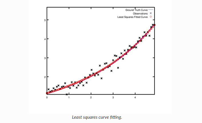
参数的初始值为m=0,c=0,代价函数为1.211734e+02。最后的解是m=0.291861,c=0.131439,代价函数值是1.056751e+00。
这些解和原始值m=0.3,c=0.1有一些细微的差别,但是是合理的(因为添加了高斯噪声)。当从噪声数据重建曲线时,我们预计会看到这样的偏差。
实际上,如果您要对m=0.3,c=0.1的目标函数进行评估,那么当目标函数值为1.082425时,拟合效果会更差。下图说明了适合度。
2.Robust Curve Fitting
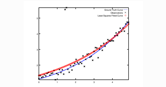
现在假设我们给出的数据有一些异常值,也就是说,我们有一些点不服从噪声模型。如果我们使用上面的代码来拟合这些数据,我们将得到如下所示的拟合结果。请注意拟合曲线是如何偏离实际情况的。
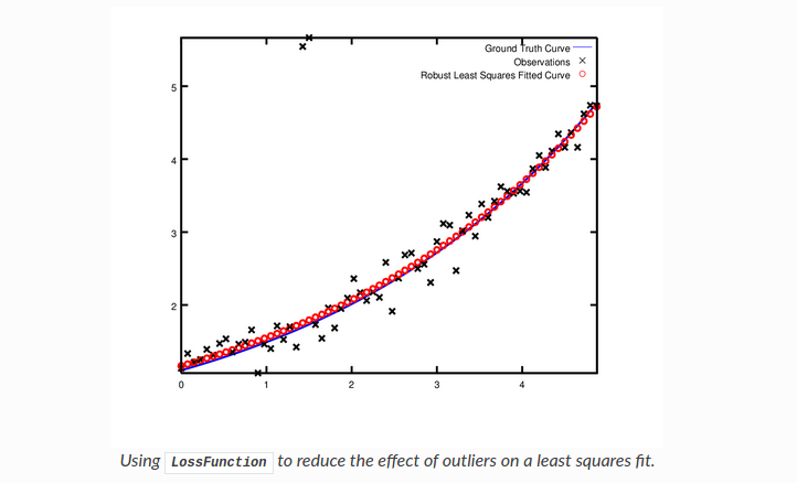
处理异常值的标准方法是使用LossFunction。损失函数降低了残差高的残差块(通常是与异常值对应的残差块)的影响。为了将损失函数与残差块联系起来,我们改变
problem.AddResidualBlock(cost_function, nullptr , &m, &c);
改变为:
problem.AddResidualBlock(cost_function, new CauchyLoss(0.5) , &m, &c);
CauchyLoss是Ceres Solver附带的损失函数之一。 参数0.5指定了损失函数的规模。拟合结果如下,通过与上图的对比,发现拟合曲线更接近真实曲线。
源代码在examples/robust_curve_fitting.cc中
#include "ceres/ceres.h"
#include "glog/logging.h"

// Data generated using the following octave code.
//   randn('seed', 23497);
//   m = 0.3;
//   c = 0.1;
//   x=[0:0.075:5];
//   y = exp(m * x + c);
//   noise = randn(size(x)) * 0.2;
//   outlier_noise = rand(size(x)) < 0.05;
//   y_observed = y + noise + outlier_noise;
//   data = [x', y_observed'];

const int kNumObservations = 67;
const double data[] = {
0.000000e+00, 1.133898e+00,
7.500000e-02, 1.334902e+00,
1.500000e-01, 1.213546e+00,
2.250000e-01, 1.252016e+00,
3.000000e-01, 1.392265e+00,
3.750000e-01, 1.314458e+00,
4.500000e-01, 1.472541e+00,
5.250000e-01, 1.536218e+00,
6.000000e-01, 1.355679e+00,
6.750000e-01, 1.463566e+00,
7.500000e-01, 1.490201e+00,
8.250000e-01, 1.658699e+00,
9.000000e-01, 1.067574e+00,
9.750000e-01, 1.464629e+00,
1.050000e+00, 1.402653e+00,
1.125000e+00, 1.713141e+00,
1.200000e+00, 1.527021e+00,
1.275000e+00, 1.702632e+00,
1.350000e+00, 1.423899e+00,
1.425000e+00, 5.543078e+00, // Outlier point
1.500000e+00, 5.664015e+00, // Outlier point
1.575000e+00, 1.732484e+00,
1.650000e+00, 1.543296e+00,
1.725000e+00, 1.959523e+00,
1.800000e+00, 1.685132e+00,
1.875000e+00, 1.951791e+00,
1.950000e+00, 2.095346e+00,
2.025000e+00, 2.361460e+00,
2.100000e+00, 2.169119e+00,
2.175000e+00, 2.061745e+00,
2.250000e+00, 2.178641e+00,
2.325000e+00, 2.104346e+00,
2.400000e+00, 2.584470e+00,
2.475000e+00, 1.914158e+00,
2.550000e+00, 2.368375e+00,
2.625000e+00, 2.686125e+00,
2.700000e+00, 2.712395e+00,
2.775000e+00, 2.499511e+00,
2.850000e+00, 2.558897e+00,
2.925000e+00, 2.309154e+00,
3.000000e+00, 2.869503e+00,
3.075000e+00, 3.116645e+00,
3.150000e+00, 3.094907e+00,
3.225000e+00, 2.471759e+00,
3.300000e+00, 3.017131e+00,
3.375000e+00, 3.232381e+00,
3.450000e+00, 2.944596e+00,
3.525000e+00, 3.385343e+00,
3.600000e+00, 3.199826e+00,
3.675000e+00, 3.423039e+00,
3.750000e+00, 3.621552e+00,
3.825000e+00, 3.559255e+00,
3.900000e+00, 3.530713e+00,
3.975000e+00, 3.561766e+00,
4.050000e+00, 3.544574e+00,
4.125000e+00, 3.867945e+00,
4.200000e+00, 4.049776e+00,
4.275000e+00, 3.885601e+00,
4.350000e+00, 4.110505e+00,
4.425000e+00, 4.345320e+00,
4.500000e+00, 4.161241e+00,
4.575000e+00, 4.363407e+00,
4.650000e+00, 4.161576e+00,
4.725000e+00, 4.619728e+00,
4.800000e+00, 4.737410e+00,
4.875000e+00, 4.727863e+00,
4.950000e+00, 4.669206e+00
};

using ceres::AutoDiffCostFunction;
using ceres::CostFunction;
using ceres::CauchyLoss;
using ceres::Problem;
using ceres::Solve;
using ceres::Solver;

struct ExponentialResidual {
  ExponentialResidual(double x, double y)
      : x_(x), y_(y) {}

  template <typename T> bool operator()(const T* const m,
                                        const T* const c,
                                        T* residual) const {
    residual[0] = y_ - exp(m[0] * x_ + c[0]);
    return true;
  }

 private:
  const double x_;
  const double y_;
};

int main(int argc, char** argv) {
  google::InitGoogleLogging(argv[0]);

  double m = 0.0;
  double c = 0.0;

  Problem problem;
  for (int i = 0; i < kNumObservations; ++i) {
    CostFunction* cost_function =
        new AutoDiffCostFunction<ExponentialResidual, 1, 1, 1>(
            new ExponentialResidual(data[2 * i], data[2 * i + 1]));
    problem.AddResidualBlock(cost_function,
                             new CauchyLoss(0.5),
                             &m, &c);
  }

  Solver::Options options;
  options.linear_solver_type = ceres::DENSE_QR;
  options.minimizer_progress_to_stdout = true;

  Solver::Summary summary;
  Solve(options, &problem, &summary);
  std::cout << summary.BriefReport() << "\n";
  std::cout << "Initial m: " << 0.0 << " c: " << 0.0 << "\n";
  std::cout << "Final   m: " << m << " c: " << c << "\n";
  return 0;
}
结果
iter      cost      cost_change  |gradient|   |step|    tr_ratio  tr_radius  ls_iter  iter_time  total_time
   0  1.815138e+01    0.00e+00    2.04e+01   0.00e+00   0.00e+00  1.00e+04        0    2.75e-04    5.29e-04
   1  2.259471e+01   -4.44e+00    0.00e+00   5.48e-01  -7.74e-01  5.00e+03        1    3.61e-05    5.99e-04
   2  2.258929e+01   -4.44e+00    0.00e+00   5.48e-01  -7.73e-01  1.25e+03        1    1.53e-05    6.21e-04
   3  2.255683e+01   -4.41e+00    0.00e+00   5.48e-01  -7.68e-01  1.56e+02        1    1.38e-05    6.41e-04
   4  2.225747e+01   -4.11e+00    0.00e+00   5.41e-01  -7.16e-01  9.77e+00        1    1.31e-05    6.59e-04
   5  1.784270e+01    3.09e-01    8.54e+01   4.72e-01   5.44e-02  5.72e+00        1    2.61e-04    9.25e-04
   6  7.557353e+00    1.03e+01    1.13e+02   1.06e-01   2.07e+00  1.72e+01        1    2.92e-04    1.22e-03
   7  2.674796e+00    4.88e+00    7.69e+01   5.41e-02   1.78e+00  5.15e+01        1    2.53e-04    1.48e-03
   8  1.946177e+00    7.29e-01    1.61e+01   5.00e-02   1.23e+00  1.54e+02        1    2.52e-04    1.74e-03
   9  1.904587e+00    4.16e-02    2.20e+00   2.64e-02   1.11e+00  4.63e+02        1    2.53e-04    2.00e-03
  10  1.902929e+00    1.66e-03    2.28e-01   6.94e-03   1.12e+00  1.39e+03        1    2.52e-04    2.26e-03
  11  1.902884e+00    4.51e-05    1.49e-02   1.27e-03   1.14e+00  4.17e+03        1    2.53e-04    2.52e-03
trust_region_minimizer.cc:707 Terminating: Function tolerance reached. |cost_change|/cost: 5.631229e-07 <= 1.000000e-06
Ceres Solver Report: Iterations: 12, Initial cost: 1.815138e+01, Final cost: 1.902884e+00, Termination: CONVERGENCE
Initial m: 0 c: 0
Final   m: 0.287605 c: 0.151213


【推荐】国内首个AI IDE,深度理解中文开发场景,立即下载体验Trae
【推荐】编程新体验,更懂你的AI,立即体验豆包MarsCode编程助手
【推荐】抖音旗下AI助手豆包,你的智能百科全书,全免费不限次数
【推荐】轻量又高性能的 SSH 工具 IShell:AI 加持,快人一步
· AI与.NET技术实操系列:基于图像分类模型对图像进行分类
· go语言实现终端里的倒计时
· 如何编写易于单元测试的代码
· 10年+ .NET Coder 心语,封装的思维:从隐藏、稳定开始理解其本质意义
· .NET Core 中如何实现缓存的预热?
· 25岁的心里话
· 闲置电脑爆改个人服务器(超详细) #公网映射 #Vmware虚拟网络编辑器
· 基于 Docker 搭建 FRP 内网穿透开源项目(很简单哒)
· 零经验选手,Compose 一天开发一款小游戏!
· 一起来玩mcp_server_sqlite,让AI帮你做增删改查!!