
HanLP — 感知机(Perceptron) -- Python
感知机
感知机是根据输入实例的特征向量 x 对其进行二类分类的线性模型:
感知机模型对应于输入空间(特征空间)中的分离超平面 $ w\cdot x+b=0 $.其中w是超平面的法向量,b是超平面的截距。
可见感知机是一种线性分类模型,属于判别模型。
感知机学习的假设
感知机学习的重要前提假设是训练数据集是线性可分的。
感知机学习策略
感知机学的策略是极小化损失函数。
损失函数的一个自然选择是误分类点的总数。但是,这样的损失函数不是参数 w, b的连续可导的函数,不易于优化。所以通常是选择误分类点到超平面 S 的总距离:
学习的策略就是求得使 L(w,b) 为最小值的 w 和 b。其中 M 是误分类点的集合。
感知机学习的算法
感知机学习算法是基于随机梯度下降法的对损失函数的最优化算法,有原始形式和对偶形式,算法简单易于实现。
原始形式
首先,任意选取一个超平面$ w_0, b_0 $,然后用梯度下降法不断地极小化目标函数。极小化的过程中不是一次使 M 中所有误分类点得梯度下降,而是一次随机选取一个误分类点,使其梯度下降。
随机选取一个误分类点$ (x_i,y_i) $,对 w,b 进行更新:
其中$ \eta(0<\eta\leq1) $是学习率。
对偶形式
对偶形式的基本想法是,将 w 和 b 表示为是咧 $ x_i $ 和标记 $ y_i $的线性组合的形式,通过求解其系数而得到 w 和 b。
逐步修改 w,b,设修改 n 次,则 w,b 关于$ (x_i,y_i) $ 的增量分别是 $ \alpha_iy_ix_i $ 和 $ \alpha_iy_i $, 这里 $ \alpha_i=n_i\eta $。最后学习到的 w,b 可以分别表示为:
这里, $ \alpha_i\geq0, i=1,2,...,N $,当 $ \eta=1 $时,表示第i个是实例点由于误分类而进行更新的次数,实例点更新次数越多,说明它距离分离超平面越近,也就越难区分,该点对学习结果的影响最大。
感知机模型对偶形式: $$f(x)=sign(\sum_{j=1}^{N}\alpha_jy_jx_j\cdot x+b) $$ 其中$$\alpha=(\alpha_1,\alpha_2,...,\alpha_N)^T$$
学习时初始化 $ \alpha \leftarrow 0, b \leftarrow 0 $, 在训练集中找分类错误的点,即:
然后更新:
知道训练集中所有点正确分类
对偶形式中训练实例仅以内积的形式出现,为了方便,可以预先将训练集中实例间的内积计算出来以矩阵的形式存储,即 Gram 矩阵。
总结
- 当训练数据集线性可分的时候,感知机学习算法是收敛的,感知机算法在训练数据集上的误分类次数 k 满足不等式:
具体证明可见 李航《统计学习方法》或 林轩田《机器学习基石》。
-
当训练当训练数据集线性可分的时候,感知机学习算法存在无穷多个解,其解由于不同的初值或不同的迭代顺序而可能不同,即存在多个分离超平面能把数据集分开。
-
感知机学习算法简单易求解,但一般的感知机算法不能解决异或等线性不可分的问题。
导入相关包并创建数据集
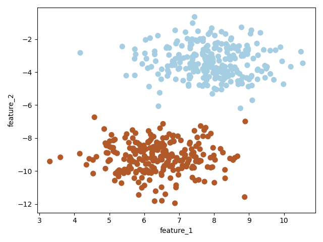
为了快速方便的创建数据集,此处采用 scikit-learn 里的 make_blobs
import numpy as np
from sklearn.datasets import make_blobs
import matplotlib.pyplot as plt
# 创建一个数据集,X有两个特征,y={-1,1}
X, y = make_blobs(n_samples=500, centers=2, random_state=6)
y[y==0] = -1
plt.scatter(X[:, 0], X[:, 1], c=y, s=30, cmap=plt.cm.Paired)
plt.xlabel("feature_1")
plt.ylabel("feature_2")
plt.show()
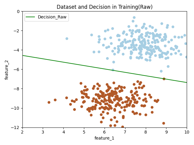
感知机(采用原始形式)
创建感知机模型的原始形式的类,并在训练集上训练,测试集上简单测试。
import numpy as np
from sklearn.datasets import make_blobs  # 为了快速方便的创建数据集,此处采用 scikit-learn 里的 make_blobs
import matplotlib.pyplot as plt

# 创建一个数据集,X有两个特征,y={-1,1}
X, y = make_blobs(n_samples=500, centers=2, random_state=6)
y[y == 0] = -1
# plt.scatter(X[:, 0], X[:, 1], c=y, s=50, cmap=plt.cm.Paired)
# plt.xlabel("feature_1")
# plt.ylabel("feature_2")
# plt.show()


class PerceptronRaw():
    def __init__(self):
        self.W = None;
        self.bias = None;

    def fit(self, x_train, y_train, learning_rate=0.05, n_iters=100, plot_train=True):
        print("开始训练...")
        num_samples, num_features = x_train.shape
        self.W = np.random.randn(num_features)
        self.bias = 0

        while True:
            erros_examples = []
            erros_examples_y = []
            # 查找错误分类的样本点
            for idx in range(num_samples):
                example = x_train[idx]
                y_idx = y_train[idx]
                # 计算距离
                distance = y_idx * (np.dot(example, self.W) + self.bias)
                if distance <= 0:
                    erros_examples.append(example)
                    erros_examples_y.append(y_idx)
            if len(erros_examples) == 0:
                break;
            else:
                print("修正参数 w => %s b => %s" % (self.W, self.bias))
                # 随机选择一个错误分类点,修正参数
                random_idx = np.random.randint(0, len(erros_examples))
                choosed_example = erros_examples[random_idx]
                choosed_example_y = erros_examples_y[random_idx]
                self.W = self.W + learning_rate * choosed_example_y * choosed_example
                self.bias = self.bias + learning_rate * choosed_example_y
        print("训练结束")

        # 绘制训练结果部分
        if plot_train is True:
            x_hyperplane = np.linspace(2, 10, 8)
            slope = -self.W[0] / self.W[1]
            intercept = -self.bias / self.W[1]
            y_hpyerplane = slope * x_hyperplane + intercept

            plt.xlabel("feature_1")
            plt.ylabel("feature_2")
            plt.xlim((2, 10))
            plt.ylim((-12, 0))
            plt.title("Dataset and Decision in Training(Raw)")
            plt.scatter(x_train[:, 0], x_train[:, 1], c=y_train, s=30, cmap=plt.cm.Paired)
            plt.plot(x_hyperplane, y_hpyerplane, color='g', label='Decision_Raw')
            plt.legend(loc='upper left')
            plt.show()

    def predict(self, x):
        if self.W is None or self.bias is None:
            raise NameError("模型未训练")
        y_predict = np.sign(np.dot(x, self.W) + self.bias)
        return y_predict


X_train = X[0:450]
y_train = y[0:450]
X_test = X[450:500]
y_test = y[450:500]

# 实例化模型,并训练
model_raw = PerceptronRaw()
model_raw.fit(X_train, y_train)


# 测试,因为测试集和训练集来自同一分布的线性可分数据集,所以这里测试准确率达到了 1.0
y_predict = model_raw.predict(X_test)

accuracy = np.sum(y_predict == y_test) / y_predict.shape[0]
print("原始形式模型在测试集上的准确率: {0}".format(accuracy))
# 原始形式模型在测试集上的准确率: 1.0
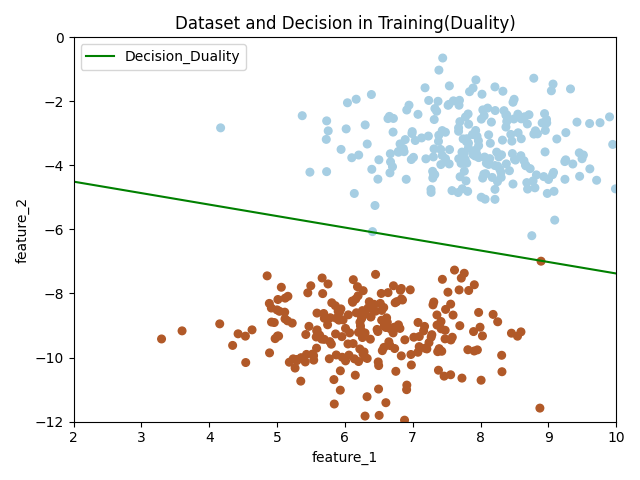
感知机(采用对偶形式)
创建感知机模型的对偶形式的类,并在训练集上训练,测试集上简单测试。
import numpy as np
from sklearn.datasets import make_blobs  # 为了快速方便的创建数据集,此处采用 scikit-learn 里的 make_blobs
import matplotlib.pyplot as plt

# 创建一个数据集,X有两个特征,y={-1,1}
X, y = make_blobs(n_samples=500, centers=2, random_state=6)
y[y == 0] = -1

# plt.scatter(X[:, 0], X[:, 1], c=y, s=50, cmap=plt.cm.Paired)
# plt.xlabel("feature_1")
# plt.ylabel("feature_2")
# plt.show()

class PerceptronDuality():
    def __init__(self):
        self.alpha = None
        self.bias = None
        self.W = None
    def fit(self, x_train, y_train, learning_rate=1, n_iters=100, plot_train=True):
        print("开始训练...")
        num_samples, num_features = x_train.shape
        self.alpha = np.zeros((num_samples,))
        self.bias = 0

        # 计算 Gram 矩阵
        gram = np.dot(x_train, x_train.T)

        while True:
            error_count = 0
            for idx in range(num_samples):
                inner_product = gram[idx]
                y_idx = y_train[idx]
                distance = y_idx * (np.sum(self.alpha * y_train * inner_product) + self.bias)
                # 如果有分类错误点,修正 alpha 和 bias,跳出本层循环,重新遍历数据计算,开始新的循环
                if distance <= 0:
                    error_count += 1
                    self.alpha[idx] = self.alpha[idx] + learning_rate
                    self.bias = self.bias + learning_rate * y_idx
                    break
            # 数据没有错分类点,跳出 while 循环
            if error_count == 0:
                break
        self.W = np.sum(self.alpha * y_train * x_train.T, axis=1)
        print("训练结束")

        # 绘制训练结果部分
        if plot_train is True:
            x_hyperplane = np.linspace(2, 10, 8)
            slope = -self.W[0]/self.W[1]
            intercept = -self.bias/self.W[1]
            y_hpyerplane = slope * x_hyperplane + intercept

            plt.xlabel("feature_1")
            plt.ylabel("feature_2")
            plt.xlim((2, 10))
            plt.ylim((-12, 0))
            plt.title("Dataset and Decision in Training(Duality)")
            plt.scatter(x_train[:, 0], x_train[:, 1], c=y_train, s=30, cmap=plt.cm.Paired)
            plt.plot(x_hyperplane, y_hpyerplane, color='g', label='Decision_Duality')
            plt.legend(loc='upper left')
            plt.show()

    def predict(self, x):
        if self.alpha is None or self.bias is None:
            raise NameError("模型未训练")
        y_predicted = np.sign(np.dot(x, self.W) + self.bias)
        return y_predicted

X_train = X[0:450]
y_train = y[0:450]
X_test = X[450:500]
y_test = y[450:500]

# 训练
model_duality = PerceptronDuality()
model_duality.fit(X_train, y_train)

# 测试
y_predict_duality = model_duality.predict(X_test)
accuracy_duality = np.sum(y_predict_duality == y_test) / y_test.shape[0]

print("对偶形式模型在测试集上的准确率: {0}".format(accuracy_duality))
#对偶形式模型在测试集上的准确率: 1.0
比较两个模型
分别从原始模型和对偶模型中获取参数,可以看出,这两个模型的分离超平面都不同,但是都能正确进行分类,这验证了总结中的结论。
当训练当训练数据集线性可分的时候,感知机学习算法存在无穷多个解,其解由于不同的初值或不同的迭代顺序而可能不同,即存在多个分离超平面能把数据集分开。
print("原始形式模型参数:")
print("W: {0}, bias: {1}".format(model_raw.W, model_raw.bias))
print()
print("对偶形式模型参数:")
print("W: {0}, bias: {1}".format(model_duality.W, model_duality.bias))
原始形式模型参数:
W: [-1.07796999 -3.05384787], bias: -11.700000000000031

对偶形式模型参数:
W: [-25.35285228 -70.71533848], bias: -268
源码: https://gitee.com/VipSoft/VipPython/tree/master/perceptron
本文来自博客园,作者:VipSoft 转载请注明原文链接:https://www.cnblogs.com/vipsoft/p/17982017

 浙公网安备 33010602011771号