
K 近邻算法 K-NearestNeighbor
理论
K-NN,即 k 近邻算法,是一种基本的分类和回归的算法,其主要思想可以归纳为:选择与待检测数据最相近的 k 个数据,再将这 k 个数据的成分最多的类别作为待测数据的类别。
假如给定数据 \(T=\{ (\pmb{x_1}, y_1), (\pmb{x_2}, y_2), \dots (\pmb{x_n}, y_n) \}\),其中 \(\pmb{x_i}\) 为数据的特征向量,\(y_i\) 为数据类别。并且 \(\pmb{x_i} \in \mathcal X \subseteq \mathbb R^n\)(\(n\) 个特征),\(y_i \in \mathcal Y = \{c_1, c_2, \dots, c_k\}\)(\(k\) 种类别)。
主要过程:
- 读入并学习已有数据
- 读入待检测数据 \(\pmb{x}\) 并输出预测类别
- 由给定距离函数 \(Dist(\pmb{x_i}, \pmb{x_j})\),在训练集中找到最近的 k 个数据,这 k 个数据记为 \(N_k(\pmb{x})\);
- 由给定分类决策函数 \(Decs(N_k(\pmb{x}))\) 得出预测类别 \(\hat y\)。
一般 \(Dist\) 采用 L2 范数,\(Decs\) 采用多数表决
def dist(x_i: ndarray, x_j:ndarray) -> ndarray:
    return sqrt((x_i - x_j) ** 2)
def desc(n_kx: ndarray) -> int:
     # n_kx记录了最近的k个点的下标
    return argmax(bincount(y_train[n_kx]))
代码仅作示意,不保证能运行
Lp 范数:
\[\begin{align*} L_p(\pmb{x_i}, \pmb{x_j})=(\sum_{l=1}^n \vert{x_i^{(l)} - x_j^{(l)}\vert}^p) ^ \frac 1 p \end{align*} \]比较特殊的是,当 \(p = \infty\) 时,有
\[\begin{align*} L_\infty(\pmb{x_i}, \pmb{x_j})=\max_{l=1}^n \vert x_i^{(l)} - x_j^{(l)}\vert \end{align*} \]
如果确定了 \(k, Dist, Decs\) 那么,k 近邻算法也就确定了。
算法
KD 树
如果采用线性扫描获取最近的 k 个点的方法,时间复杂度为 \(O(n)\),但采用 KD 树的数据结构,可以达到 \(O(\log n)\)。
KD 树,顾名思义是一种树结构。可以将常见的二叉搜索树推而广之,二叉搜索树分叉时只考虑一个维度。如果拓展到 n 个维度就能获得 KD 树。
不妨取 \(\pmb{x} = (x^{(1)}, x^{(2)}, \dots, x^{(n)})\),有 n 个维度。
构造
- 第一次分叉:使用 \(x^{(1)}\)$ 划分,对 \(x_i \in \mathcal X\),\(x_i^{(1)} < m\) 的在左子树,\(x_i^{(1)} \ge m\) 的在右子树。\(m\) 为划分点,一般取 \(x_i^{(1)}\) 的中位数,\(m\) 所属的 \(\pmb{x}_0\) 为该节点的值;
- 第二次分叉:使用 \(x^{(2)}\) 划分;
- …………;
- 第 n 次分叉:使用 \(x^{(n)}\) 划分;
- 第 n + 1 次分叉:使用 \(x^{(1)}\) 划分(回到 1 了);
- …………。
也就是说,对深度为 \(j\) 的节点使用 \(x^{((j \mod n) + 1)}\) 划分。
要注意的是,只有分叉后子树中的有多个数据时才需要继续分叉。
搜索
在某个节点结点被分为三个部分:当前结点(\(\pmb{x}_0\)、\(m\))、左子树、右子树。如果已经有 k 个结点已经在左子树被找全,那么就分析 \(\pmb{x}\) 与 \(m\) 的距离,如果此距离小于 k 个结点与 \(\pmb x\) 的最大距离,那么说明当前节点和右子树都可能有更近的结点,于是在右子树继续查找;反之,则不需要查找,直接回答上一个结点即可。
现在所有空间都已经被 KD 树划分了,当输入数据 \(\pmb{x}\) 时,依照如下步骤找到最近的 k 个数据:
定义函数 get_knn(self, node, i, point, k) 为能够在以 node 为当前节点,当前节点深度为 i 的 KD 树(可能是子树)中找到 point 的 k 个最近邻的算法。假设已经有全局变量 result = [] 作为 k 近邻的容器, 下面使用递归的方法实现 get_knn()。
- 首先在这个 KD 树中找到 \(\pmb{x}\) 所属于的叶节点,小于的走左子树,大于的走右子树,这一点和二叉树搜索类似,不过每深一层,所使用的维度就移动到下一个。直到最底层,也就是叶节点;
- 从当前结点向上查找,访问过的结点将会被标记,只有没有访问过得结点才需要采取子步骤;
- 将当前结点插入
result,按与point的距离排好序,长度超过k的部分将会被切除。 - 查看父节点
prev,如果prev == null说明当前节点为整个 KD 树的根节点,结束。 - 否则,判断要不要检查右子树(即对右子树使用
get_knn(),右子树!= null),以下为要的情况:result长度不足k;result中的最远距离比prev的左右子树的划分线(\(m\)) 和point的距离大。
- 当前结点移动到父节点
prev。
- 将当前结点插入
实现
用 Python 实现 KD 树
class Node:
    def __init__(self, value, prev=None, left=None, right=None):
        self.value = value
        self.prev = prev
        self.left, self.right = left, right
        self.marked = False

    def distance(self, other):
        """
        计算与other的距离
        """
        return np.sqrt(np.sum((self.value - other.value) ** 2))

    def segment(self, other, i) -> float:
        """
        计算与other的间隔,即第i个数据的差的绝对值
        """
        return abs(self.value[i] - other.value[i])


class KDTree:

    def __init__(self, values: np.ndarray):
        self.length = values.shape[1]
        self.root = self._init(values, 0)

    def _init(self, values: np.ndarray, i: int) -> Node:
        """
        递归地初始化KD树
        """
        count = values.shape[0]
        if count == 0:
            return None

        # 按第i个值的顺序排序并划分
        values = values[values[:, i].argsort()]
        median = count // 2
        i = (i + 1) % self.length
        node = Node(values[median], None,
                    self._init(values[:median], i),
                    self._init(values[median+1:], i))

        if node.left:
            node.left.prev = node
        if node.right:
            node.right.prev = node
        return node

    def get_knn(self, value: np.ndarray, k: int) -> np.ndarray:
        """
        调用_get_knn()
        """
        nodes = []
        point = Node(value)

        self._get_knn(nodes, self.root, point, k, 0)
        self.refresh(self.root)

        return np.array([n[1].value for n in nodes])

    def _get_knn(self, out: list, node: Node, point: Node, k: int, i: int) -> None:
        while node:
            prev = node
            if point.value[i] < node.value[i]:
                node = node.left
            else:
                node = node.right
            i = (i + 1) % self.length
        j = (i + self.length - 1) % self.length

        node = prev

        while node:
            prev = node.prev

            if node.marked:
                node = prev
                continue

            node.marked = True
            self.insert_nearest(out, point, node, k)

            if prev is None:
                return

            i = j
            j = (i + self.length - 1) % self.length
            sibling = prev.right if node is prev.left else prev.left

            if sibling and (len(out) != k or point.segment(prev, j) < out[-1][0]):
                self._get_knn(out, sibling, point, k, i)

    def insert_nearest(self, out: list, point: Node, node: Node, k: int) -> None:
        """
        在out中按与point的距离插入node,并保证len(out) <= k
        """
        dist = point.distance(node)
        for i, n in enumerate(out):
            if n[0] >= dist:
                out.insert(i, (dist, node))
                break
        else:
            out.append((dist, node))
        if len(out) > k:
            out.pop()

    def refresh(self, node) -> None:
        """
        将所有结点的访问标记清除
        """
        if node:
            node.marked = False
            self.refresh(node.left)
            self.refresh(node.right)

    def layer_scan(self) -> None:
        """
        层序遍历,观察KD树
        """
        node = self.root

        nodes = [node]
        children = []

        while nodes:
            for node in nodes:
                if node:
                    print(node.value, end=' ')
                    children += [node.left, node.right]
                else:
                    print('null', end=' ')
            print()
            nodes, children = children, []
应用
鸢尾花数据集
用经典的鸢尾花数据集做简单测试。
观测数据
import matplotlib.pyplot as plt
import numpy as np
import pandas as pd
from sklearn.datasets import load_iris

iris_dataset = load_iris()
print(iris_dataset.keys())
print(iris_dataset.feature_names)
dict_keys(['data', 'target', 'frame', 'target_names', 'DESCR', 'feature_names', 'filename'])

['sepal length (cm)',
 'sepal width (cm)',
 'petal length (cm)',
 'petal width (cm)']
有四个特征,三种类别。
X, y = iris_dataset.data, iris_dataset.target
dataframe = pd.DataFrame(X, columns=iris_dataset.feature_names)
plot_mat = pd.plotting.scatter_matrix(dataframe, c=y, figsize=(15, 15), marker='o',
                                      hist_kwds={'bins': 20}, cmap='tab10')
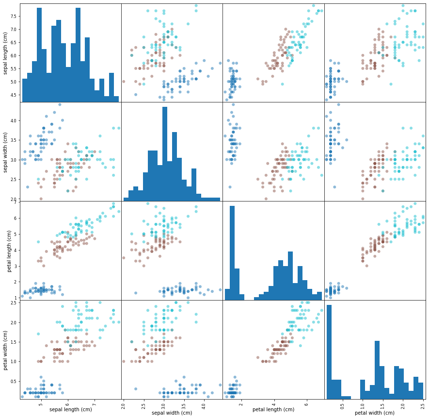
可以看出,较深的蓝色代表的数据会比较容易与较浅的青色和棕色分开。
应用算法
from sklearn.neighbors import KNeighborsClassifier
from sklearn.model_selection import train_test_split

X_train, X_test, y_train, y_test = train_test_split(X, y)
print(X_train.shape, X_test.shape, y_train.shape, y_test.shape)
# (112, 4) (38, 4) (112,) (38,)
使用 k = 3 测试
knn = KNeighborsClassifier(n_neighbors=3)
knn.fit(X_train, y_train)
print(knn.score(X_test, y_test)) # 正确率0.9473684210526315
使用不同 k 值并绘图
training_acc = []
test_acc = []
ns = list(range(1, 60))
for n in ns:
    model = KNeighborsClassifier(n_neighbors=n).fit(X_train, y_train)
    training_acc.append(model.score(X_train, y_train))
    test_acc.append(model.score(X_test, y_test))

plt.plot(ns, training_acc, label='training')
plt.plot(ns, test_acc, label='test')
plt.legend()
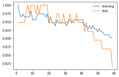
开始时 k 较小,模型复杂度大,容易受噪声影响,过拟合;
随着 k 的增加,training 数据下降,test 上升,泛化能力变好;
k 达到一定程度,模型复杂度小,容易忽略数据中的有用信息,欠拟合。
过拟合:训练数据表现好,测试数据表现差;
欠拟合:训练数据和测试数据表现都差。
我们追求的就是测试数据表现要好,也就是泛化能力强的意思。
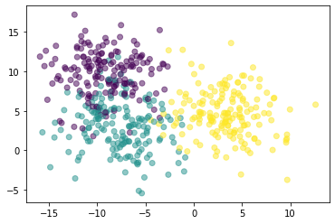
二维图像实例
使用 sklearn.datasets.make_blobs() 作离散点数据:
n_samples数据个数;n_features数据特征,这里有x,y两个轴作特征;cluster_std数据集的标准差,控制不同类别的数据的离散程度。
from sklearn.datasets import make_blobs

X, y = make_blobs(n_samples=500, n_features=2, cluster_std=3.0)
plt.scatter(X[:,0], X[:,1], c=y, alpha=0.5)
X_train, X_test, y_train, y_test = train_test_split(X, y)
print(X_train.shape, X_test.shape, y_train.shape, y_test.shape)
# (375, 2) (125, 2) (375,) (125,)
contourf(x, y, z) 本来是作为画等高线的函数,此次由于预测值是离散值,自然也可以使用。
x, y, z分别为 x 坐标,y 坐标,高度
# 获得数据范围
eps = X_train.std() / 2
x_min, x_max = X_train[:, 0].min() - eps, X_train[:, 0].max() + eps
y_min, y_max = X_train[:, 1].min() - eps, X_train[:, 1].max() + eps

# 铺满数据AB
a = np.linspace(x_min, x_max, 500)
b = np.linspace(y_min, y_max, 500)

A, B = np.meshgrid(a, b)
AB = np.hstack((A.reshape(-1, 1), B.reshape(-1, 1)))

# 四个图像
fig, axes = plt.subplots(1, 4, figsize=(18, 5))

# 预测AB
for n, ax in zip([1, 5, 10, 100], axes):
    model = KNeighborsClassifier(n_neighbors=n).fit(X_train, y_train)
    ax.contourf(A, B, model.predict(AB).reshape(A.shape), alpha=0.2)
    ax.set_title(f'{n} neighbor(s)')
    ax.scatter(X[:,0], X[:,1], c=y, alpha=0.5)

# 绘图
plt.xlim(x_min, x_max)
plt.ylim(y_min, y_max)
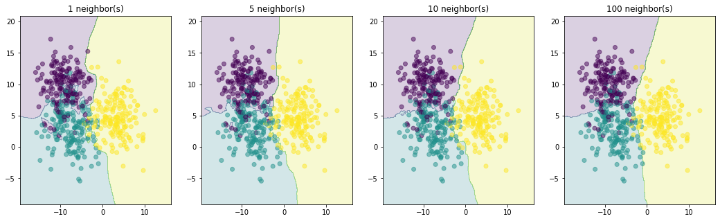
结论:随着 k 的增加,图像分界线也变得更平滑了。
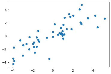
一维数据实例
使用 numpy.random.multivariate_normal() 产生数据
mean:均值,n维分布的平均值;cov:分布的协方差矩阵,必须是对称的和正半定的;size样本的大小,依numpy惯例,也可以是数组之类的。
mean 的长度和 cov 的维数必须相等。
data = np.random.multivariate_normal(mean=[0, 0], cov=[[5, 4], [4, 5]], size=50)
X, y = data[:,0].reshape(-1, 1), data[:,1]
plt.scatter(X, y)
from sklearn.neighbors import KNeighborsRegressor

eps = X.std() / 2
x_min, x_max = X.min() - eps, X.max() + eps

xx = np.linspace(x_min, x_max, 500).reshape(-1, 1)

fig, axes = plt.subplots(1, 4, figsize=(18, 5))

for n, ax in zip([1, 2, 5, 9], axes):
    yy = KNeighborsRegressor(n_neighbors=n).fit(X, y).predict(xx)
    ax.scatter(X, y, alpha=0.8)
    ax.plot(xx, yy, alpha=0.8, c='r')
    ax.set_title(f'{n} neighbor(s)')

plt.xlim(x_min, x_max)
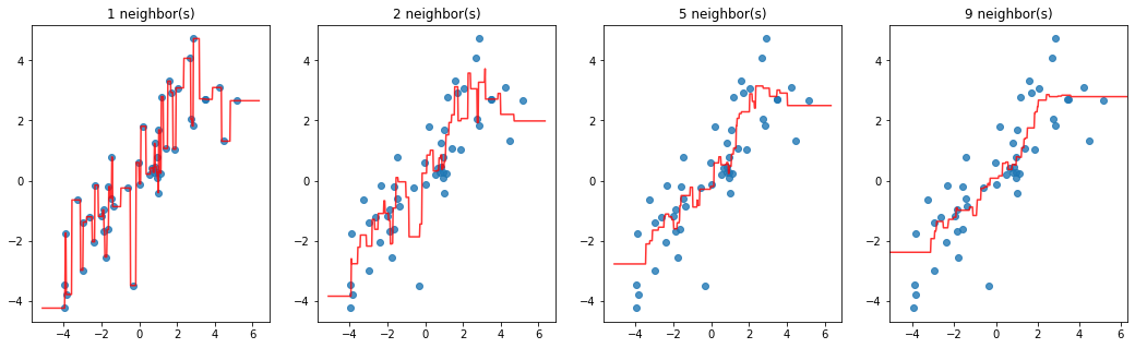
k 较小时发生了过拟合。
在图像的左右两侧,预测值变为一条直线,这是因为最近的 k 个数据已经不会变化了。
参考书目及网站
- 《统计学习方法(第二版)》
- 《Python机器学习基础教程》Introduction to Machine Learning with Python
- scikit-learn api
- numpy doc

 浙公网安备 33010602011771号