Sample Means（耶鲁大学教材）

Sample Means

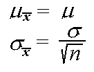
The sample mean from a group of observations is an estimate of the population mean. Given a sample of sizen, consider n independent random variables X₁,X₂, ..., X_n, each corresponding to one randomly selected observation. Each of these variables has the distribution of the population, with mean and standard deviation. The sample mean is defined to be.
By the properties of means and variances of random variables, the mean and variance of the sample mean are the following:

Although the mean of the distribution of is identical to the mean of the population distribution, the variance is much smaller for large sample sizes.

For example, suppose the random variable X records a randomly selected student's score on a national test, where the population distribution for the score is normal with mean 70 and standard deviation 5 (N(70,5)). Given asimple random sample (SRS) of 200 students, the distribution of the sample mean score has mean 70 and standard deviation 5/sqrt(200) = 5/14.14 = 0.35.

Distribution of the Sample Mean

When the distribution of the population is normal, then the distribution of the sample mean is also normal. For a normal population distribution with mean and standard deviation, the distribution of the sample mean is normal, with mean and standard deviation.

This result follows from the fact that any linear combination of independent normal random variables is also normally distributed. This means that for two independent normal random variablesX and Y and any constants a and b, aX + bY will be normally distributed. In the case of the sample mean, the linear combination is =(1/n)*(X₁ + X₂ + ... X_n).

For example, consider the distributions of yearly average test scores on a national test in two areas of the country. In the first area, the test scoreX is normally distributed with mean 70 and standard deviation 5. In the second area, the yearly average test scoreY is normally distributed with mean 65 and standard deviation 8. The differenceX - Y between the two areas is normally distributed, with mean 70-65 = 5 and variance 5² + 8² = 25 + 64 = 89. The standard deviation is the square root of the variance, 9.43. The probability that areaX will have a higher score than area Y may be calculated as follows:
P(X > Y) = P(X - Y > 0)
= P(((X - Y) - 5)/9.43 > (0 - 5)/9.43)
= P(Z > -0.53) = 1 - P(Z < -0.53) = 1 - 0.2981 = 0.7019.
Area X will have a higher average score than area Y about 70% of the time.

The Central Limit Theorem

The most important result about sample means is the Central Limit Theorem. Simply stated, this theorem says that for a large enough sample sizen, the distribution of the sample mean will approach a normal distribution.This is true for a sample of independent random variables from any population distribution, as long as the population has a finite standard deviation.

A formal statement of the Central Limit Theorem is the following:

If is the mean of a random sampleX₁, X₂, ... , X_n of size n from a distribution with a finite mean and a finite positive variance², then the distribution ofW = isN(0,1) in the limit as n approaches infinity.

This means that the variable is distributedN(,).

One well-known application of this theorem is the normal approximation to the binomial distribution.

Example

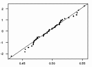
Using the MINITAB "RANDOM" command with the "UNIFORM" subcommand, I generated 100 samples of size 50 each from the Uniform(0,1) distribution. The mean of this distribution is 0.5, and its standard deviation is approximately 0.3. I then applied the "RMEAN" command to calculate the sample mean across the rows of my sample, resulting in 50 sample mean values (each of which represents the mean of 100 observations). The MINITAB "DESCRIBE" command gave the following information about the sample mean data:

Descriptive Statistics


Variable        N     Mean   Median  Tr Mean    StDev  SE Mean
C101           50  0.49478  0.49436  0.49450  0.02548  0.00360

Variable      Min      Max       Q1       Q3
C101      0.43233  0.55343  0.47443  0.51216      

The mean 0.49 is nearly equal to the population mean 0.5. The desired value for the standard deviation is the population standard deviation divided by the square root of the size of the sample (which is 10 in this case), approximately 0.3/10 = 0.03. The calculated value for this sample is 0.025. To evaluate the normality of the sample mean data, I used the "NSCORES" and "PLOT" commands to create a normal quantile plot of the data, shown below.

The plot indicates that the data follow an approximately normal distribution, lying close to a diagonal line through the main body of the points.