从DDPM到DDIM (一) 极大似然估计与证据下界
现在网络上关于DDPM和DDIM的讲解有很多,但无论什么样的讲解,都不如自己推到一遍来的痛快。笔者希望就这篇文章,从头到尾对扩散模型做一次完整的推导。本文的很多部分都参考了 Calvin Luo 和 Stanley Chan 写的经典教程。也推荐大家取阅读学习。
DDPM是一个双向马尔可夫模型,其分为扩散过程和采样过程。
扩散过程是对于图片不断加噪的过程,每一步添加少量的高斯噪声,直到图像完全变为纯高斯噪声。为什么逐步添加小的高斯噪声,而不是一步到位,直接添加很强的噪声呢?这一点我们留到之后来探讨。
采样过程则相反,是对纯高斯噪声图像不断去噪,逐步恢复原始图像的过程。
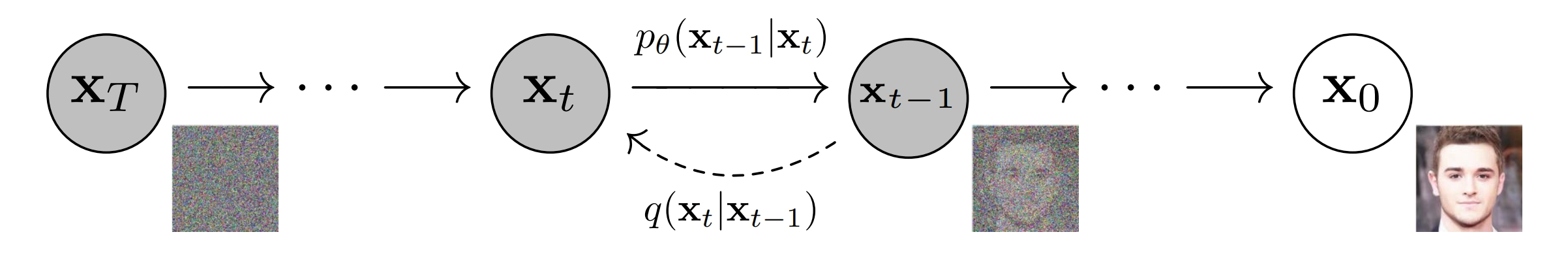
下图展示了DDPM原文中的马尔可夫模型。
![img]()
其中\(\mathbf{x}_T\)代表纯高斯噪声,\(\mathbf{x}_t, 0 < t < T\) 代表中间的隐变量, \(\mathbf{x}_0\) 代表生成的图像。从 \(\mathbf{x}_0\) 逐步加噪到 \(\mathbf{x}_T\) 的过程是不需要神经网络参数的,简单地讲高斯噪声和图像或者隐变量进行线性组合即可,单步加噪过程用\(q(\mathbf{x}_t | \mathbf{x}_{t-1})\)来表示。但是去噪的过程,我们是不知道的,这里的单步去噪过程,我们用 \(p_{\theta}(\mathbf{x}_{t-1} | \mathbf{x}_{t})\) 来表示。之所以这里增加一个 \(\theta\) 下标,是因为 \(p_{\theta}(\mathbf{x}_{t-1} | \mathbf{x}_{t})\) 是用神经网络来逼近的转移概率, \(\theta\) 代表神经网络参数。
扩散模型首先需要大量的图片进行训练,训练的目标就是估计图像的概率分布。训练完毕后,生成图像的过程就是在计算出的概率分布中采样。因此生成模型一般都有训练算法和采样算法,VAE、GAN、diffusion,还有如今大火的大预言模型(LLM)都不例外。本文讨论的DDPM和DDIM在训练方法上是一样的,只是DDIM在采样方法上与前者有所不同。
估计生成样本的概率分布的最经典的方法就是极大似然估计,我们从极大似然估计开始。
1、从极大似然估计开始
首先简单回顾一下概率论中的一些基本概念,边缘概率密度、联合概率密度、概率乘法公式和马尔可夫链,最后回顾一个强大的数学工具:Jenson 不等式。对这些熟悉的同学可以不需要看1.1节。
1.1、概念回顾
边缘概率密度和联合概率密度: 大家可能还记得概率论中的边缘概率密度,忘了也不要紧,我们简单回顾一下。对于二维随机变量\((X, Y)\),其联合概率密度函数是\(f(x, y)\),那么我不管\(Y\),单看\(X\)的概率密度,就是\(X\)的边缘概率密度,其计算方式如下:
\[\begin{aligned}
f_{X}(t) = \int_{-\infty}^{\infty} f(x, y) d y \\
\end{aligned} \\
\]
概率乘法公式: 对于联合概率\(P(A_1 A_2 ... A_{n})\),若\(P(A_1 A_2 ... A_{n-1}) 0\),则:
\[\begin{aligned}
P(A_1 A_2 ... A_{n}) &= P(A_1 A_2 ... A_{n-1}) P(A_n | A_1 A_2 ... A_{n-1}) \\
&= P(A_1) P(A_2 | A_1) P(A_3 | A_1 A_2) ... P(A_n | A_1 A_2 ... A_{n-1})
\end{aligned} \\
\]
概率乘法公式可以用条件概率的定义和数学归纳法证明。
马尔可夫链定义: 随机过程 \(\left\{X_n, n = 0,1,2,...\right\}\)称为马尔可夫链,若随机过程在某一时刻的随机变量 \(X_n\) 只取有限或可列个值(比如非负整数集,若不另外说明,以集合 \(\mathcal{S}\) 来表示),并且对于任意的 \(n \geq 0\) ,及任意状态 \(i, j, i_0, i_1, ..., i_{n-1} \in \mathcal{S}\),有
\[\begin{aligned}
P(X_{n+1} = j | X_{0} = i_{0}, X_{1} = i_{1}, ... X_{n} = i) = P(X_{n+1} = j | X_{n} = i) \\
\end{aligned} \\
\]
其中 \(X_n = i\) 表示过程在时刻 \(n\) 处于状态 \(i\)。称 \(\mathcal{S}\) 为该过程的状态空间。上式刻画了马尔可夫链的特性,称为马尔可夫性。
Jenson 不等式。Jenson 不等式有多种形式,我们这里采用其积分形式:
若 \(f(x)\) 为凸函数,另一个函数 \(q(x)\) 满足:
\[\int_{-\infty}^{\infty} q(x) d x = 1 \\
\]
则有:
\[f \left[ \int_{-\infty}^{\infty} q(x) x d x \right] \leq \int_{-\infty}^{\infty} q(x) f(x) d x \\
\]
更进一步地,若 \(x\) 为随机变量 \(X\) 的取值,\(q(x)\) 为随机变量 \(X\) 的概率密度函数,则 Jenson不等式为:
\[f \left[ \mathbb{E}(x) \right] \leq \mathbb{E}[f(x)] \\
\]
关于 Jenson 不等式的证明,用凸函数的定义证明即可。网上有很多,这里不再赘述。
1.2、概率分布表示
生成模型的主要目标是估计需要生成的数据的概率分布。这里就是\(p\left(\mathbf{x}_0\right)\),如何估计\(p\left(\mathbf{x}_0\right)\)呢。一个比较直接的想法就是把\(p\left(\mathbf{x}_0\right)\)当作整个马尔可夫模型的边缘概率:
\[\begin{aligned}
p\left(\mathbf{x}_0\right) = \int p\left(\mathbf{x}_{0:T}\right) d \mathbf{x}_{1:T} \\
\end{aligned} \\
\]
这里\(p\left(\mathbf{x}_{0:T}\right)\)表示\(\mathbf{x}_{0}, \mathbf{x}_{1}, ..., \mathbf{x}_{T}\) 多个随机变量的联合概率分布。\(d \mathbf{x}_{1:T}\) 表示对\(\mathbf{x}_{1}, \mathbf{x}_{2}, ..., \mathbf{x}_{T}\) 这 \(T\) 个随机变量求多重积分。
显然,这个积分很不好求。Sohl-Dickstein等人在2015年的扩散模型的开山之作中,采用的是这个方法:
\[\begin{aligned}
p\left(\mathbf{x}_0\right) &= \int p\left(\mathbf{x}_{0:T}\right) \textcolor{blue}{\frac{q\left(\mathbf{x}_{1:T} | \mathbf{x}_{0}\right)}{q\left(\mathbf{x}_{1:T} | \mathbf{x}_{0}\right)}} d \mathbf{x}_{1:T} \quad\quad 积分内部乘1\\
&= \int \textcolor{blue}{q\left(\mathbf{x}_{1:T} | \mathbf{x}_{0}\right)} \frac{p\left(\mathbf{x}_{0:T}\right)}{\textcolor{blue}{q\left(\mathbf{x}_{1:T} | \mathbf{x}_{0}\right)}} d \mathbf{x}_{1:T} \\
&= \mathbb{E}_{\textcolor{blue}{q\left(\mathbf{x}_{1:T} | \mathbf{x}_{0}\right)}} \left[\frac{p\left(\mathbf{x}_{0:T}\right)}{\textcolor{blue}{q\left(\mathbf{x}_{1:T} | \mathbf{x}_{0}\right)}}\right] \quad\quad随机变量函数的期望\\
\end{aligned} \tag{1}
\]
Sohl-Dickstein等人借鉴的是统计物理中的技巧:退火重要性采样(annealed importance sampling) 和 Jarzynski equality。这两个就涉及到笔者的知识盲区了,感兴趣的同学可以自行找相关资料学习。(果然数学物理基础不牢就搞不好科研~)。
这里有的同学可能会有疑问,为什么用分子分母都为 \(q\left(\mathbf{x}_{1:T} | \mathbf{x}_{0}\right)\) 的因子乘进去?这里笔者尝试给出另一种解释,就是我们在求边缘分布的时候,可以尝试将联合概率分布拆开,然后想办法乘一个已知的并且与其类似的项,然后将这些项分别放在分子与分母的位置,让他们分别进行比较。因为这是KL散度的形式,而KL散度是比较好算的。\(q\left(\mathbf{x}_{1:T} | \mathbf{x}_{0}\right)\) 的好处就是也可以按照贝叶斯公式和马尔可夫性质拆解成多个条件概率的连乘积,这些条件概率与 \(p\left(\mathbf{x}_{0:T}\right)\) 拆解之后的条件概率几乎可以一一对应,而且每个条件概率表示的都是扩散过程的单步转移概率,这我们都是知道的。那么为什么不用 \(q\left(\mathbf{x}_{0:T}\right)\) 呢?其实 \(p\) 和 \(q\) 本质上是一种符号,\(q\left(\mathbf{x}_{0:T}\right)\) 和 \(p\left(\mathbf{x}_{0:T}\right)\) 其实表示的是一个东西。
这里自然就引出了问题,这么一堆随机变量的联合概率密度,我们还是不知道啊,\(p\left(\mathbf{x}_{0:T}\right)\) 和 \(q\left(\mathbf{x}_{1:T} | \mathbf{x}_{0}\right)\) 如何该表示?
利用概率乘法公式,有:
\[\begin{aligned}
p\left(\mathbf{x}_{0:T}\right) &= p\left(\mathbf{x}_{T}\right) p\left(\mathbf{x}_{T-1}|\mathbf{x}_{T}\right) p\left(\mathbf{x}_{T-2}|\mathbf{x}_{T-1},\mathbf{x}_{T}\right) ... p\left(\mathbf{x}_{0}|\mathbf{x}_{1:T}\right)\\
\end{aligned} \tag{2}
\]
我们这里是单独把 \(p\left(\mathbf{x}_{T}\right)\),单独提出来,这是因为 \(\mathbf{x}_{T}\) 服从高斯分布,这是我们知道的分布;如果反方向的来表示,这么表示的话:
\[\begin{aligned}
p\left(\mathbf{x}_{0:T}\right) &= p\left(\mathbf{x}_{0}\right) p\left(\mathbf{x}_{1}|\mathbf{x}_{0}\right) p\left(\mathbf{x}_{2}|\mathbf{x}_{1},\mathbf{x}_{0}\right) ... p\left(\mathbf{x}_{T}|\mathbf{x}_{0:T-1}\right)\\
\end{aligned} \tag{3}
\]
(3)式这样表示明显不如(2)式,因为我们最初就是要求 \(p\left(\mathbf{x}_{0}\right)\) ,而计算(3)式则需要知道 \(p\left(\mathbf{x}_{0}\right)\),这样就陷入了死循环。因此学术界采用(2)式来对联合概率进行拆解。
因为扩散模型是马尔可夫链,某一时刻的随机变量只和前一个时刻有关,所以:
\[\begin{aligned}
p\left(\mathbf{x}_{t-1}|\mathbf{x}_{\leq t}\right) = p\left(\mathbf{x}_{t-1}|\mathbf{x}_{t}\right)\\
\end{aligned} \\
\]
于是有:
\[\begin{aligned}
p\left(\mathbf{x}_{0:T}\right) = p\left(\mathbf{x}_{T}\right) \prod_{t=1}^{T} p\left(\mathbf{x}_{t-1}|\mathbf{x}_{t}\right)\\
\end{aligned} \\
\]
文章一开始说到,在扩散模型的采样过程中,单步转移概率是不知道的,需要用神经网络来拟合,所以我们给采样过程的单步转移概率都加一个下标 \(\theta\),这样就得到了最终的联合概率:
\[\begin{aligned}
\textcolor{blue}{p\left(\mathbf{x}_{0:T}\right) = p\left(\mathbf{x}_{T}\right) \prod_{t=1}^{T} p_{\theta}\left(\mathbf{x}_{t-1}|\mathbf{x}_{t}\right)}
\end{aligned} \tag{4}
\]
类似地,我们来计算 \(q\left(\mathbf{x}_{1:T} | \mathbf{x}_{0}\right)\) 的拆解表示:
\[\begin{aligned}
q\left(\mathbf{x}_{1:T} | \mathbf{x}_{0}\right) &= q\left(\mathbf{x}_{1} | \mathbf{x}_{0}\right) q\left(\mathbf{x}_{2} | \mathbf{x}_{0:1}\right) ... q\left(\mathbf{x}_{T} | \mathbf{x}_{0:T-1}\right) \quad\quad 概率乘法公式\\
&= \prod_{t=1}^T q\left(\mathbf{x}_{t} | \mathbf{x}_{t-1}\right) \quad\quad 马尔可夫性质\\
\end{aligned} \\
\]
于是得到了以\(\mathbf{x}_0\) 为条件的扩散过程的联合概率分布:
\[\begin{aligned}
\textcolor{blue}{q\left(\mathbf{x}_{1:T} | \mathbf{x}_{0}\right) = \prod_{t=1}^T q\left(\mathbf{x}_{t} | \mathbf{x}_{t-1}\right)} \\
\end{aligned} \tag{5}
\]
数学推导的一个很重要的事情就是分清楚哪些是已知量,哪些是未知量。\(q\left(\mathbf{x}_{t} | \mathbf{x}_{t-1}\right)\) 是已知的,因为根据扩散模型的定义,\(q\left(\mathbf{x}_{t} | \mathbf{x}_{t-1}\right)\) 是服从高斯分布的;另外 \(p\left(\mathbf{x}_{T} \right)\) 也是已知的,因为 \(\mathbf{x}_{T}\) 代表的是纯高斯噪声,因此 \(p\left(\mathbf{x}_{T} \right)\) 也是服从高斯分布的。
1.3、极大似然估计
既然我们知道了\(p\left(\mathbf{x}_{0:T}\right)\) 和 \(q\left(\mathbf{x}_{1:T} | \mathbf{x}_{0}\right)\) 的表达式,我们可以继续对 (1) 式进行化简了。首先我们要对(1)式进行缩放,(1)式我们难以计算,我们可以计算(1)式的下界,然后极大化它的下界就相当于极大化(1)式了。这确实是一种巧妙的方法,这个方法在VAE推导的时候就已经用过了,大家不懂VAE也没关系,我们在这里重新推导一遍。
计算(1)式的下界一般有两种办法。分别是Jenson不等式法和KL散度方法。下面我们分别给出两种方法的推导。
Jenson不等式法。在进行极大似然估计的时候,一般会对概率分布取对数,于是我们对(1)式取对数可得:
\[\begin{aligned}
\log p\left(\mathbf{x}_0\right) &= \log \int p\left(\mathbf{x}_{0:T}\right) {\frac{q\left(\mathbf{x}_{1:T} | \mathbf{x}_{0}\right)}{q\left(\mathbf{x}_{1:T} | \mathbf{x}_{0}\right)}} d \mathbf{x}_{1:T}\\
&= \log \int {q\left(\mathbf{x}_{1:T} | \mathbf{x}_{0}\right)} \frac{p\left(\mathbf{x}_{0:T}\right)}{{q\left(\mathbf{x}_{1:T} | \mathbf{x}_{0}\right)}} d \mathbf{x}_{1:T} \\
&= \log \left\{\mathbb{E}_{{q\left(\mathbf{x}_{1:T} | \mathbf{x}_{0}\right)}} \left[\frac{p\left(\mathbf{x}_{0:T}\right)}{{q\left(\mathbf{x}_{1:T} | \mathbf{x}_{0}\right)}}\right] \right\}\\
&\geq \mathbb{E}_{q\left(\mathbf{x}_{1:T} | \mathbf{x}_{0}\right)} \left[ \log \frac{p\left(\mathbf{x}_{0:T}\right)}{{q\left(\mathbf{x}_{1:T} | \mathbf{x}_{0}\right)}}\right] \quad\quad \text{Jenson不等式,log()为concave函数}\\
&= \mathcal{L}
\end{aligned}
\]
\(\mathcal{L} = \mathbb{E}_{q\left(\mathbf{x}_{1:T} | \mathbf{x}_{0}\right)} \left[ \log \frac{p\left(\mathbf{x}_{0:T}\right)}{{q\left(\mathbf{x}_{1:T} | \mathbf{x}_{0}\right)}}\right]\) 被称为随机变量 \(\mathbf{x}_0\) 的证据下界 (Evidence Lower BOund, ELBO)。
KL散度方法。当然,我们也可以不采用Jenson不等式,利用KL散度的非负性,同样也可以得出证据下界。将证据下界中的数学期望展开,写为积分形式为:
\[\begin{aligned}
\mathcal{L} = \int {q\left(\mathbf{x}_{1:T} | \mathbf{x}_{0}\right)} \log \frac{p\left(\mathbf{x}_{0:T}\right)}{{q\left(\mathbf{x}_{1:T} | \mathbf{x}_{0}\right)}} d \mathbf{x}_{1:T}\\
\end{aligned}
\]
另外,我们定义一个KL散度:
\[\begin{aligned}
\text{KL}\left(q\left(\mathbf{x}_{1:T} | \mathbf{x}_{0}\right) || p\left(\mathbf{x}_{1:T} | \mathbf{x}_{0}\right)\right) = \int q\left(\mathbf{x}_{1:T} | \mathbf{x}_{0}\right) \log \frac{q\left(\mathbf{x}_{1:T} | \mathbf{x}_{0}\right)}{p\left(\mathbf{x}_{1:T} | \mathbf{x}_{0}\right)} d \mathbf{x}_{1:T}\\
\end{aligned}
\]
下面我们将验证:
\[\begin{aligned}
\log p\left(\mathbf{x}_0\right) &= \mathcal{L} + \text{KL}\left(q\left(\mathbf{x}_{1:T} | \mathbf{x}_{0}\right) || p\left(\mathbf{x}_{1:T} | \mathbf{x}_{0}\right)\right)\\
\end{aligned} \tag{6}
\]
具体地,有:
\[\begin{aligned}
\mathcal{L} + \text{KL}\left(q\left(\mathbf{x}_{1:T} | \mathbf{x}_{0}\right) || p\left(\mathbf{x}_{1:T} | \mathbf{x}_{0}\right)\right) &= \int q\left(\mathbf{x}_{1:T} | \mathbf{x}_{0}\right) \log \frac{p\left(\mathbf{x}_{0:T}\right)}{p\left(\mathbf{x}_{1:T} | \mathbf{x}_{0}\right)} d \mathbf{x}_{1:T}\\
&= \int q\left(\mathbf{x}_{1:T} | \mathbf{x}_{0}\right) \log \frac{p\left(\mathbf{x}_{1:T} | \mathbf{x}_{0}\right) p\left(\mathbf{x}_{0}\right)}{p\left(\mathbf{x}_{1:T} | \mathbf{x}_{0}\right)} d \mathbf{x}_{1:T}\\
&= \int q\left(\mathbf{x}_{1:T} | \mathbf{x}_{0}\right) \log p\left(\mathbf{x}_{0}\right) d \mathbf{x}_{1:T}\\
&= \log p\left(\mathbf{x}_{0}\right) \int q\left(\mathbf{x}_{1:T} | \mathbf{x}_{0}\right) d \mathbf{x}_{1:T} \quad\quad 概率密度积分为1\\
&= \log p\left(\mathbf{x}_{0}\right)\\
\end{aligned}
\]
因此,(6)式成立。由于\(\text{KL}\left(q\left(\mathbf{x}_{1:T} | \mathbf{x}_{0}\right) || p\left(\mathbf{x}_{1:T} | \mathbf{x}_{0}\right)\right) \geq 0\),所以:
\[\log p\left(\mathbf{x}_{0}\right) \geq \mathcal{L}
\]
个人还是更喜欢Jenson不等式法,因为此方法的思路一气呵成;而KL散度法像是先知道最终的答案,然后取验证答案的正确性。而且KL的非负性也是可以用Jenson不等式证明的,所以二者在数学原理上本质是一样的。KL散度法有一个优势,就是能让我们知道 \(\log p\left(\mathbf{x}_{0}\right)\) 与证据下界的差距有多大,二者仅仅相差一个KL散度:\(\text{KL}\left(q\left(\mathbf{x}_{1:T} | \mathbf{x}_{0}\right) || p\left(\mathbf{x}_{1:T} | \mathbf{x}_{0}\right)\right)\)。关于这两个概率分布的物理意义,笔者认为可以这样理解:\(q\left(\mathbf{x}_{1:T} | \mathbf{x}_{0}\right)\) 是真实的,在给定图片 \(\mathbf{x}_0\) 作为条件下的前向联合概率,而 \(p\left(\mathbf{x}_{1:T} | \mathbf{x}_{0}\right)\) 是我们估计的条件前向联合概率。而KL散度描述的是两个概率分布之间的距离,如果我们估计的比较准确的话,二者的距离是比较小的。因此这也印证了我们采用证据下界来替代 \(\log p\left(\mathbf{x}_0\right)\) 做极大似然估计的合理性。
下面,我们的方向就是逐步简化证据下界,直到简化为我们编程可实现的形式。
2、简化证据下界
对证据下界的化简,需要用到三个我们之前推导出来的表达式。为了方便阅读,我们把(4)式,(5)式,还有证据下界重写到这里。
\[\begin{aligned}
\textcolor{blue}{p\left(\mathbf{x}_{0:T}\right) = p\left(\mathbf{x}_{T}\right) \prod_{t=1}^{T} p_{\theta}\left(\mathbf{x}_{t-1}|\mathbf{x}_{t}\right)}
\end{aligned} \tag{4}
\]
\[\begin{aligned}
\textcolor{blue}{q\left(\mathbf{x}_{1:T} | \mathbf{x}_{0}\right) = \prod_{t=1}^T q\left(\mathbf{x}_{t} | \mathbf{x}_{t-1}\right)} \\
\end{aligned} \tag{5}
\]
\[\begin{aligned}
\textcolor{blue}{\mathcal{L} = \mathbb{E}_{q\left(\mathbf{x}_{1:T} | \mathbf{x}_{0}\right)} \left[ \log \frac{p\left(\mathbf{x}_{0:T}\right)}{{q\left(\mathbf{x}_{1:T} | \mathbf{x}_{0}\right)}}\right]}\\
\end{aligned} \tag{7}
\]
下面我们将(4)式和(5)式代入到(7)式中,有:
\[\begin{aligned}
\mathcal{L} &= \mathbb{E}_{q\left(\mathbf{x}_{1:T} | \mathbf{x}_{0}\right)} \left[ \log \frac{p\left(\mathbf{x}_{0:T}\right)}{{q\left(\mathbf{x}_{1:T} | \mathbf{x}_{0}\right)}}\right]\\
&= \mathbb{E}_{q\left(\mathbf{x}_{1:T} | \mathbf{x}_{0}\right)} \left[ \log \frac{p\left(\mathbf{x}_{T}\right) \prod_{t=1}^{T} p_{\theta}\left(\mathbf{x}_{t-1}|\mathbf{x}_{t}\right)}{\prod_{t=1}^T q\left(\mathbf{x}_{t} | \mathbf{x}_{t-1}\right)}\right]\\
&= \mathbb{E}_{q\left(\mathbf{x}_{1:T} | \mathbf{x}_{0}\right)} \left[ \log \frac{p\left(\mathbf{x}_{T}\right) p_{\theta}\left(\mathbf{x}_{0}|\mathbf{x}_{1}\right) \prod_{t=2}^{T} p_{\theta}\left(\mathbf{x}_{t-1}|\mathbf{x}_{t}\right)}{\prod_{t=1}^T q\left(\mathbf{x}_{t} | \mathbf{x}_{t-1}\right)}\right]\\
&= \mathbb{E}_{q\left(\mathbf{x}_{1:T} | \mathbf{x}_{0}\right)} \left[ \log \frac{p\left(\mathbf{x}_{T}\right) p_{\theta}\left(\mathbf{x}_{0}|\mathbf{x}_{1}\right) \prod_{t=1}^{T-1} \textcolor{blue}{p_{\theta}\left(\mathbf{x}_{t}|\mathbf{x}_{t+1}\right)}}{\prod_{t=1}^T \textcolor{blue}{q\left(\mathbf{x}_{t} | \mathbf{x}_{t-1}\right)}}\right] \\
\end{aligned}
\]
蓝色部分的操作,是将分子分母的表示的随机变量概率保持一致,对同一个随机变量的概率分布的描述才具备可比性。而且,我们希望分子分母的连乘号下标保持一致,这样才能进一步化简。下面我们继续:
\[\begin{aligned}
\mathcal{L} &= \mathbb{E}_{q\left(\mathbf{x}_{1:T} | \mathbf{x}_{0}\right)} \left[ \log \frac{p\left(\mathbf{x}_{T}\right) p_{\theta}\left(\mathbf{x}_{0}|\mathbf{x}_{1}\right) \prod_{t=1}^{T-1} \textcolor{blue}{p_{\theta}\left(\mathbf{x}_{t}|\mathbf{x}_{t+1}\right)}}{\prod_{t=1}^T \textcolor{blue}{q\left(\mathbf{x}_{t} | \mathbf{x}_{t-1}\right)}}\right] \\
&= \mathbb{E}_{q\left(\mathbf{x}_{1:T} | \mathbf{x}_{0}\right)} \left[ \log \frac{p\left(\mathbf{x}_{T}\right) p_{\theta}\left(\mathbf{x}_{0}|\mathbf{x}_{1}\right) \prod_{t=1}^{T-1} {p_{\theta}\left(\mathbf{x}_{t}|\mathbf{x}_{t+1}\right)}}{q\left(\mathbf{x}_{T} | \mathbf{x}_{T-1}\right) \prod_{t=1}^{T-1} {q\left(\mathbf{x}_{t} | \mathbf{x}_{t-1}\right)}}\right] \\
&= \mathbb{E}_{q\left(\mathbf{x}_{1:T} | \mathbf{x}_{0}\right)} \left[ \log \frac{p\left(\mathbf{x}_{T}\right) p_{\theta}\left(\mathbf{x}_{0}|\mathbf{x}_{1}\right)}{q\left(\mathbf{x}_{T} | \mathbf{x}_{T-1}\right) }\right] + \mathbb{E}_{q\left(\mathbf{x}_{1:T} | \mathbf{x}_{0}\right)} \left[ \log \prod_{t=1}^{T-1} \frac{p_{\theta}\left(\mathbf{x}_{t}|\mathbf{x}_{t+1}\right)}{q\left(\mathbf{x}_{t} | \mathbf{x}_{t-1}\right)} \right]\\
&= \textcolor{skyblue}{\mathbb{E}_{q\left(\mathbf{x}_{1:T} | \mathbf{x}_{0}\right)} \left[ \log p_{\theta}\left(\mathbf{x}_{0}|\mathbf{x}_{1}\right) \right]} + \textcolor{darkred}{\mathbb{E}_{q\left(\mathbf{x}_{1:T} | \mathbf{x}_{0}\right)} \left[ \log \frac{p\left(\mathbf{x}_{T}\right)}{q\left(\mathbf{x}_{T} | \mathbf{x}_{T-1}\right)} \right]} + \textcolor{darkgreen}{\sum_{t=1}^{T-1} \mathbb{E}_{q\left(\mathbf{x}_{1:T} | \mathbf{x}_{0}\right)} \left[ \log \frac{p_{\theta}\left(\mathbf{x}_{t}|\mathbf{x}_{t+1}\right)}{q\left(\mathbf{x}_{t} | \mathbf{x}_{t-1}\right)} \right]} \\
\end{aligned} \tag{8}
\]
上式第一项,第二项,第三项分别被称为 重建项(Reconstruction Term)、先验匹配项(Prior Matching Term)、一致项(Consistency Term)。
- 重建项。顾名思义,这是对最后构图的预测概率。给定预测的最后一个隐变量 \(\mathbf{x}_1\),预测生成的图像 \(\mathbf{x}_0\) 的对数概率。
- 先验匹配项。 这一项描述的是扩散过程的最后一步生成的高斯噪声与纯高斯噪声的相似度,因为这一项并没有神经网络参数,所以不需要优化,后续网络训练的时候可以将这一项舍去。
- 一致项。这一项描述的是采样过程的单步转移概率 \(p_{\theta}\left(\mathbf{x}_{t}|\mathbf{x}_{t+1}\right)\) 和扩散过程的单步转移概率 \(q\left(\mathbf{x}_{t}|\mathbf{x}_{t-1}\right)\) 的距离。由于 \(q\left(\mathbf{x}_{t}|\mathbf{x}_{t-1}\right)\) 是服从高斯分布的(加噪过程自己定义的),所以我们希望采样过程的单步转移概率 \(p_{\theta}\left(\mathbf{x}_{t}|\mathbf{x}_{t+1}\right)\) 也服从高斯分布,这样才能使得二者的KL散度更加接近。我们之后会看到,最小化二者的KL散度等价于最大似然估计。
到这里我们通过观察可以发现,乘上 \(q\left(\mathbf{x}_{1:T} | \mathbf{x}_{0}\right)\),的期望中,存在很多无关的随机变量,因此这三项可以进一步化简。以上式重建项为例,我们将上式重建项写成积分形式:
\[\begin{aligned}
\mathbb{E}_{q\left(\mathbf{x}_{1:T} | \mathbf{x}_{0}\right)} \left[ \log p_{\theta}\left(\mathbf{x}_{0}|\mathbf{x}_{1}\right) \right] = \int q\left(\mathbf{x}_{1:T} | \mathbf{x}_{0}\right) \log p_{\theta}\left(\mathbf{x}_{0}|\mathbf{x}_{1}\right) \textcolor{blue}{d \mathbf{x}_{0:T}}
\end{aligned}
\]
可能有的同学搞不清楚积分微元是哪个变量,如果不知道的话就把所有的随机变量都算为积分微元。如果哪个微元不需要的话,是可以被积分积掉的。注意到,\(\mathbf{x}_0\) 是真实图像,而不是随机变量,所以随机变量最多就是 \(\mathbf{x}_{1:T}\)。 具体我们来看:
\[\begin{aligned}
\textcolor{Skyblue}{\mathbb{E}_{q\left(\mathbf{x}_{1:T} | \mathbf{x}_{0}\right)} \left[ \log p_{\theta}\left(\mathbf{x}_{0}|\mathbf{x}_{1}\right) \right]} &= \int q\left(\mathbf{x}_{1:T} | \mathbf{x}_{0}\right) p_{\theta}\left(\mathbf{x}_{0}|\mathbf{x}_{1}\right) \textcolor{blue}{d \mathbf{x}_{1:T}} \\
&= \int \int ... \int q\left(\mathbf{x}_{1:T} | \mathbf{x}_{0}\right) \log p_{\theta}\left(\mathbf{x}_{0}|\mathbf{x}_{1}\right) \textcolor{blue}{d \mathbf{x}_{1} d \mathbf{x}_{2} ... d \mathbf{x}_{T}} \\
&= \int \log p_{\theta}\left(\mathbf{x}_{0}|\mathbf{x}_{1}\right) \textcolor{blue}{\left[\int ... \int q\left(\mathbf{x}_{1:T} | \mathbf{x}_{0}\right) d \mathbf{x}_{2} d \mathbf{x}_{3} ... d \mathbf{x}_{T} \right]}d \mathbf{x}_{1} \\
&= \int \log p_{\theta}\left(\mathbf{x}_{0}|\mathbf{x}_{1}\right) \textcolor{blue}{q\left(\mathbf{x}_{1} | \mathbf{x}_{0}\right) }d \mathbf{x}_{1} \\
&= \mathbb{E}_{q\left(\mathbf{x}_{1} | \mathbf{x}_{0}\right)} \left[ \log p_{\theta}\left(\mathbf{x}_{0}|\mathbf{x}_{1}\right) \right]
\end{aligned}
\]
类似地,我们看 先验匹配项 和 一致项。先验匹配项中除了 \(\mathbf{x}_T\) 和 \(\mathbf{x}_{T-1}\) 这两个随机变量之外,其他的随机变量都会被积分积掉,于是就是:
\[\begin{aligned}
\textcolor{Darkred}{\mathbb{E}_{q\left(\mathbf{x}_{1:T} | \mathbf{x}_{0}\right)} \left[ \log \frac{p\left(\mathbf{x}_{T}\right)}{q\left(\mathbf{x}_{T} | \mathbf{x}_{T-1}\right)} \right]} &= \int q\left(\mathbf{x}_{1:T} | \mathbf{x}_{0}\right) \log \frac{p\left(\mathbf{x}_{T}\right)}{q\left(\mathbf{x}_{T} | \mathbf{x}_{T-1}\right)} d \mathbf{x}_{1:T}\\
&= \int q\left(\mathbf{x}_{T-1}, \mathbf{x}_{T} | \mathbf{x}_{0}\right) \log \frac{p\left(\mathbf{x}_{T}\right)}{q\left(\mathbf{x}_{T} | \mathbf{x}_{T-1}\right)} d \mathbf{x}_{T-1} d\mathbf{x}_{T}\\
&= \mathbb{E}_{q\left(\mathbf{x}_{T-1}, \mathbf{x}_{T} | \mathbf{x}_{0}\right)} \left[ \log \frac{p\left(\mathbf{x}_{T}\right)}{q\left(\mathbf{x}_{T} | \mathbf{x}_{T-1}\right)} \right]\\
\end{aligned}
\]
一致项也用类似的操作:
\[\begin{aligned}
\textcolor{Darkgreen}{\sum_{t=1}^{T-1} \mathbb{E}_{q\left(\mathbf{x}_{1:T} | \mathbf{x}_{0}\right)} \left[ \log \frac{p_{\theta}\left(\mathbf{x}_{t}|\mathbf{x}_{t+1}\right)}{q\left(\mathbf{x}_{t} | \mathbf{x}_{t-1}\right)} \right]} &= \sum_{t=1}^{T-1} \int q\left(\mathbf{x}_{1:T} | \mathbf{x}_{0}\right) \log \frac{p_{\theta}\left(\mathbf{x}_{t}|\mathbf{x}_{t+1}\right)}{q\left(\mathbf{x}_{t} | \mathbf{x}_{t-1}\right)} d \mathbf{x}_{1:T}\\
&= \sum_{t=1}^{T-1} \int q\left(\mathbf{x}_{t-1}, \mathbf{x}_{t}, \mathbf{x}_{t+1} | \mathbf{x}_{0}\right) \log \frac{p_{\theta}\left(\mathbf{x}_{t}|\mathbf{x}_{t+1}\right)}{q\left(\mathbf{x}_{t} | \mathbf{x}_{t-1}\right)} d \mathbf{x}_{t-1} d \mathbf{x}_{t} d \mathbf{x}_{t+1}\\
&= \sum_{t=1}^{T-1} \mathbb{E}_{q\left(\mathbf{x}_{t-1}, \mathbf{x}_{t}, \mathbf{x}_{t+1} | \mathbf{x}_{0}\right)} \left[ \log \frac{p_{\theta}\left(\mathbf{x}_{t}|\mathbf{x}_{t+1}\right)}{q\left(\mathbf{x}_{t} | \mathbf{x}_{t-1}\right)} \right]
\end{aligned}
\]
下面我们继续化简,化简乘KL散度的形式。因为两个高斯分布的KL散度可以写成二范数Loss的形式,这是我们编程可实现的。我们先给出KL散度的定义。设两个概率分布和 \(Q\) 和 \(P\),在连续随机变量的情况下,他们的概率密度函数分别为 \(q(x)\) \(p(x)\),那么二者的KL散度为:
\[\begin{aligned}
\mathbb{D}_{\text{KL}}\left(Q || P\right) = - \int q(x) \log \frac{p(x)}{q(x)} dx
\end{aligned}
\]
注意,KL散度没有对称性,即 \(\text{KL}\left(Q || P\right)\) 和 \(\text{KL}\left(P || Q\right)\) 是不同的。
下面,我们以 一致项 中的其中一项为例子,来写成KL散度形式:
\[\begin{aligned}
\textcolor{darkgreen}{\mathbb{E}_{q\left(\mathbf{x}_{t-1}, \mathbf{x}_{t}, \mathbf{x}_{t+1} | \mathbf{x}_{0}\right)} \left[ \log \frac{p_{\theta}\left(\mathbf{x}_{t}|\mathbf{x}_{t+1}\right)}{q\left(\mathbf{x}_{t} | \mathbf{x}_{t-1}\right)} \right]} &= \int q\left(\mathbf{x}_{t-1}, \mathbf{x}_{t}, \mathbf{x}_{t+1} | \mathbf{x}_{0}\right) \log \frac{p_{\theta}\left(\mathbf{x}_{t}|\mathbf{x}_{t+1}\right)}{q\left(\mathbf{x}_{t} | \mathbf{x}_{t-1}\right)} d \mathbf{x}_{t-1} d \mathbf{x}_{t} d \mathbf{x}_{t+1} \\
&= \int \textcolor{red}{q\left(\mathbf{x}_{t-1}, \mathbf{x}_{t+1} | \mathbf{x}_{0}\right) q\left(\mathbf{x}_{t} | \mathbf{x}_{t-1}\right)} \log \frac{p_{\theta}\left(\mathbf{x}_{t}|\mathbf{x}_{t+1}\right)}{q\left(\mathbf{x}_{t} | \mathbf{x}_{t-1}\right)} d \mathbf{x}_{t-1} d \mathbf{x}_{t} d \mathbf{x}_{t+1} \\
&= \int q\left(\mathbf{x}_{t-1}, \mathbf{x}_{t+1} | \mathbf{x}_{0}\right) \left\{\int q\left(\mathbf{x}_{t} | \mathbf{x}_{t-1}\right) \log \frac{p_{\theta}\left(\mathbf{x}_{t}|\mathbf{x}_{t+1}\right)}{q\left(\mathbf{x}_{t} | \mathbf{x}_{t-1}\right)} d \mathbf{x}_{t} \right\} d \mathbf{x}_{t-1} d \mathbf{x}_{t+1} \\
&= - \int q\left(\mathbf{x}_{t-1}, \mathbf{x}_{t+1} | \mathbf{x}_{0}\right) \mathbb{D}_{\text{KL}}\left(q\left(\mathbf{x}_{t} | \mathbf{x}_{t-1}\right) || p_{\theta}\left(\mathbf{x}_{t}|\mathbf{x}_{t+1}\right)\right) d \mathbf{x}_{t-1} d \mathbf{x}_{t+1} \\
&= - \mathbb{E}_{q\left(\mathbf{x}_{t-1}, \mathbf{x}_{t+1} | \mathbf{x}_{0}\right)} \left[ \mathbb{D}_{\text{KL}}\left(q\left(\mathbf{x}_{t} | \mathbf{x}_{t-1}\right) || p_{\theta}\left(\mathbf{x}_{t}|\mathbf{x}_{t+1}\right)\right) \right] \\
\end{aligned}
\]
上式红色的部分,是参考的开篇提到的那两个教程。笔者自己推了一下,并没有得出相应的结果。
如果有好的解释,欢迎讨论。不过这里是否严格并不重要,之后我们会解释,事实上我们使用的是另外一种推导方式。
类似地,先验匹配项 也可以用类似的方法表示成KL散度的形式:
\[\begin{aligned}
\textcolor{Darkred}{\mathbb{E}_{q\left(\mathbf{x}_{T-1}, \mathbf{x}_{T} | \mathbf{x}_{0}\right)} \left[ \log \frac{p\left(\mathbf{x}_{T}\right)}{q\left(\mathbf{x}_{T} | \mathbf{x}_{T-1}\right)} \right]} &= \int q\left(\mathbf{x}_{T-1}, \mathbf{x}_{T} | \mathbf{x}_{0}\right) \log \frac{p\left(\mathbf{x}_{T}\right)}{q\left(\mathbf{x}_{T} | \mathbf{x}_{T-1}\right)} d \mathbf{x}_{T-1} d\mathbf{x}_{T}\\
&= \int \textcolor{red}{q\left(\mathbf{x}_{T-1} | \mathbf{x}_{0}\right) q\left(\mathbf{x}_{T} | \mathbf{x}_{T-1}\right)} \log \frac{p\left(\mathbf{x}_{T}\right)}{q\left(\mathbf{x}_{T} | \mathbf{x}_{T-1}\right)} d \mathbf{x}_{T-1} d\mathbf{x}_{T}\\
&= \int q\left(\mathbf{x}_{T-1} | \mathbf{x}_{0}\right) \left\{\int q\left(\mathbf{x}_{T} | \mathbf{x}_{T-1}\right) \log \frac{p\left(\mathbf{x}_{T}\right)}{q\left(\mathbf{x}_{T} | \mathbf{x}_{T-1}\right)} d \mathbf{x}_{T} \right\} d\mathbf{x}_{T-1}\\
&= - \int q\left(\mathbf{x}_{T-1} | \mathbf{x}_{0}\right) \mathbb{D}_{\text{KL}}\left(q\left(\mathbf{x}_{T} | \mathbf{x}_{T-1}\right) || p\left(\mathbf{x}_{T}\right)\right) d\mathbf{x}_{T-1}\\
&= - \mathbb{E}_{q\left(\mathbf{x}_{T-1} | \mathbf{x}_{0}\right)} \left[ \mathbb{D}_{\text{KL}}\left(q\left(\mathbf{x}_{T} | \mathbf{x}_{T-1}\right) || p\left(\mathbf{x}_{T}\right)\right) \right] \\
\end{aligned}
\]
这里红色的部分,我们可以详细验证一下:
\[\begin{aligned}
q\left(\mathbf{x}_{T-1} | \mathbf{x}_{0}\right) q\left(\mathbf{x}_{T} | \mathbf{x}_{T-1}\right) &= q\left(\mathbf{x}_{T-1} | \mathbf{x}_{0}\right) q\left(\mathbf{x}_{T} | \mathbf{x}_{T-1}, \mathbf{x}_{0}\right) \quad\quad 马尔可夫性质 \\
&= q\left(\mathbf{x}_{T-1}, \mathbf{x}_{T} | \mathbf{x}_{0}\right) \quad\quad 条件概率公式 \\
\end{aligned}
\]
没有什么问题。
下面我们整理一下结果。我们简化的证据下界为:
\[\begin{aligned}
\mathcal{L} = \textcolor{skyblue}{\mathbb{E}_{q\left(\mathbf{x}_{1:T} | \mathbf{x}_{0}\right)} \left[ \log p_{\theta}\left(\mathbf{x}_{0}|\mathbf{x}_{1}\right) \right]} &- \textcolor{darkred}{\mathbb{E}_{q\left(\mathbf{x}_{T-1} | \mathbf{x}_{0}\right)} \left[ \mathbb{D}_{\text{KL}}\left(q\left(\mathbf{x}_{T} | \mathbf{x}_{T-1}\right) || p\left(\mathbf{x}_{T}\right)\right) \right]} \\
&- \textcolor{darkgreen}{\sum_{t=1}^{T-1} \mathbb{E}_{q\left(\mathbf{x}_{t-1}, \mathbf{x}_{t+1} | \mathbf{x}_{0}\right)} \left[ \mathbb{D}_{\text{KL}}\left(q\left(\mathbf{x}_{t} | \mathbf{x}_{t-1}\right) || p_{\theta}\left(\mathbf{x}_{t}|\mathbf{x}_{t+1}\right)\right) \right]} \\
\end{aligned} \tag{9}
\]
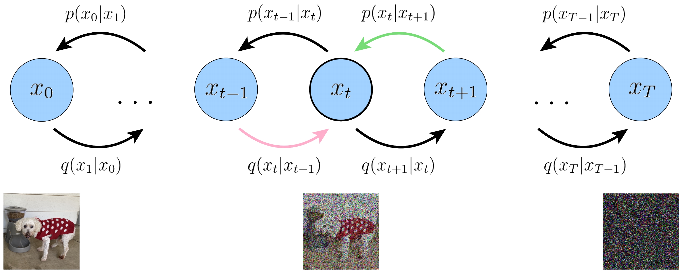
我们看第三项,也就是 一致项。我们发现两个概率分布 \(q\left(\mathbf{x}_{t} | \mathbf{x}_{t-1}\right)\) 和 \(p_{\theta}\left(\mathbf{x}_{t}|\mathbf{x}_{t+1}\right)\) 有时序上的错位,如下图展示的粉色线和绿色线。这相当于最小化两个错一位的概率分布,这显然不是我们希望的结果。虽然错一位影响也不大,但总归是不完美的。而且,这两个转移概率的方向也不一样。因此,下面我们就要想办法对证据下界进行优化,看看能不能推导出两个在时序上完全对齐的两个概率分布的KL散度。
![img]()
如何优化证据下界呢。我们放到下一篇文章中来讲:
从DDPM到DDIM (二) 前向过程与反向过程的概率分布。


 浙公网安备 33010602011771号